INTEGRATE Timing Analysis Example¶

This example demonstrates how to perform comprehensive timing analysis of the INTEGRATE workflow using the built-in timing_compute() and timing_plot() functions.

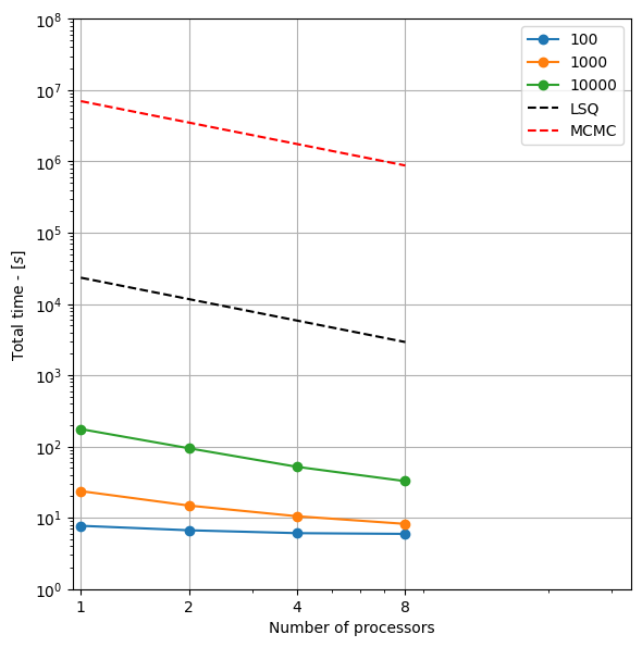
The timing analysis benchmarks four main components:

Prior model generation (layered geological models)
Forward modeling using GA-AEM electromagnetic simulation
Rejection sampling for Bayesian inversion
Posterior statistics computation

Results are automatically saved and comprehensive plots are generated showing:

Performance scaling with dataset size and processor count
Speedup analysis and parallel efficiency
Comparisons with traditional least squares and MCMC methods
Component-wise timing breakdowns

[1]:

try:
    # Check if the code is running in an IPython kernel (which includes Jupyter notebooks)
    get_ipython()
    # If the above line doesn't raise an error, it means we are in a Jupyter environment
    # Execute the magic commands using IPython's run_line_magic function
    get_ipython().run_line_magic('load_ext', 'autoreload')
    get_ipython().run_line_magic('autoreload', '2')
except:
    # If get_ipython() raises an error, we are not in a Jupyter environment
    pass

[2]:

import integrate as ig
import numpy as np
import matplotlib.pyplot as plt
import time

# Check if parallel computations can be performed
parallel = ig.use_parallel(showInfo=1)

Notebook detected. Parallel processing is OK

Quick Timing Test¶

This example runs a quick timing test with a small subset of dataset sizes and processor counts to demonstrate the timing functions.

[3]:

print("# Running Quick Timing Test")
print("="*50)

# Define test parameters - small arrays for quick demonstration
N_arr_quick = [100, 1000, 10000]  # Small dataset sizes for quick test
Nproc_arr_quick = [1, 2, 4, 8]     # Limited processor counts

# Run timing computation
timing_file = ig.timing_compute(N_arr=N_arr_quick, Nproc_arr=Nproc_arr_quick)

print(f"\nTiming results saved to: {timing_file}")

# Running Quick Timing Test
==================================================
Notebook detected. Parallel processing is OK
# TIMING TEST
Hostname (system): d52534 (Linux)
Number of processors: 24
Using data file: DAUGAARD_AVG.h5
Using GEX file: TX07_20231016_2x4_RC20-33.gex
Testing on 3 data sets of size(s): [100, 1000, 10000]
Testing on 4 sets of core(s): [1, 2, 4, 8]
Writing results to timing_d52534-Linux-24core_Nproc4_N3.npz
=====================================================
TIMING: N=100, Ncpu=1, Ncpu_min=0
=====================================================

File PRIOR_CHI2_NF_5_log-uniform_N100.h5 does not exist.
Using file_basename=TX07_20231016_2x4_RC20-33
prior_data_gaaem: Using 1 parallel threads.

prior_data_gaaem: Time=  1.8s/100 soundings. 18.4ms/sounding, 54.5it/s

integrate_rejection: Time=  1.0s/11693 soundings,  0.1ms/sounding, 11573.6it/s. T_av=2437.2, EV_av=-727.3

=====================================================
TIMING: N=1000, Ncpu=1, Ncpu_min=0
=====================================================

File PRIOR_CHI2_NF_5_log-uniform_N1000.h5 does not exist.
Using file_basename=TX07_20231016_2x4_RC20-33
prior_data_gaaem: Using 1 parallel threads.

prior_data_gaaem: Time= 15.9s/1000 soundings. 15.9ms/sounding, 62.9it/s

integrate_rejection: Time=  2.4s/11693 soundings,  0.2ms/sounding, 4936.4it/s. T_av=349.5, EV_av=-242.1

=====================================================
TIMING: N=10000, Ncpu=1, Ncpu_min=1
=====================================================

File PRIOR_CHI2_NF_5_log-uniform_N10000.h5 does not exist.
Using file_basename=TX07_20231016_2x4_RC20-33
prior_data_gaaem: Using 1 parallel threads.

prior_data_gaaem: Time=155.3s/10000 soundings. 15.5ms/sounding, 64.4it/s

integrate_rejection: Time= 14.4s/11693 soundings,  1.2ms/sounding, 813.2it/s. T_av=104.4, EV_av=-130.3

=====================================================
TIMING: N=100, Ncpu=2, Ncpu_min=0
=====================================================

Using file_basename=TX07_20231016_2x4_RC20-33
prior_data_gaaem: Using 2 parallel threads.

prior_data_gaaem: Time=  1.1s/100 soundings. 10.8ms/sounding, 92.4it/s

integrate_rejection: Time=  0.6s/11693 soundings,  0.1ms/sounding, 19315.3it/s. T_av=2323.4, EV_av=-642.7

=====================================================
TIMING: N=1000, Ncpu=2, Ncpu_min=0
=====================================================

Using file_basename=TX07_20231016_2x4_RC20-33
prior_data_gaaem: Using 2 parallel threads.

prior_data_gaaem: Time=  8.3s/1000 soundings.  8.3ms/sounding, 120.7it/s

integrate_rejection: Time=  1.2s/11693 soundings,  0.1ms/sounding, 9387.0it/s. T_av=344.0, EV_av=-253.2

=====================================================
TIMING: N=10000, Ncpu=2, Ncpu_min=1
=====================================================

Using file_basename=TX07_20231016_2x4_RC20-33
prior_data_gaaem: Using 2 parallel threads.

prior_data_gaaem: Time= 80.5s/10000 soundings.  8.0ms/sounding, 124.3it/s

integrate_rejection: Time=  8.0s/11693 soundings,  0.7ms/sounding, 1458.2it/s. T_av=104.9, EV_av=-131.6

=====================================================
TIMING: N=100, Ncpu=4, Ncpu_min=0
=====================================================

Using file_basename=TX07_20231016_2x4_RC20-33
prior_data_gaaem: Using 4 parallel threads.

prior_data_gaaem: Time=  0.7s/100 soundings.  7.1ms/sounding, 141.3it/s

integrate_rejection: Time=  0.4s/11693 soundings,  0.0ms/sounding, 30370.0it/s. T_av=2456.2, EV_av=-856.0

=====================================================
TIMING: N=1000, Ncpu=4, Ncpu_min=0
=====================================================

Using file_basename=TX07_20231016_2x4_RC20-33
prior_data_gaaem: Using 4 parallel threads.

prior_data_gaaem: Time=  4.3s/1000 soundings.  4.3ms/sounding, 230.4it/s

integrate_rejection: Time=  0.7s/11693 soundings,  0.1ms/sounding, 16435.1it/s. T_av=366.5, EV_av=-270.1

=====================================================
TIMING: N=10000, Ncpu=4, Ncpu_min=1
=====================================================

Using file_basename=TX07_20231016_2x4_RC20-33
prior_data_gaaem: Using 4 parallel threads.

prior_data_gaaem: Time= 40.9s/10000 soundings.  4.1ms/sounding, 244.5it/s

integrate_rejection: Time=  5.1s/11693 soundings,  0.4ms/sounding, 2290.8it/s. T_av=104.8, EV_av=-129.3

=====================================================
TIMING: N=100, Ncpu=8, Ncpu_min=0
=====================================================

Using file_basename=TX07_20231016_2x4_RC20-33
prior_data_gaaem: Using 8 parallel threads.

prior_data_gaaem: Time=  0.5s/100 soundings.  5.4ms/sounding, 184.6it/s

integrate_rejection: Time=  0.3s/11693 soundings,  0.0ms/sounding, 34569.5it/s. T_av=2497.2, EV_av=-710.5

=====================================================
TIMING: N=1000, Ncpu=8, Ncpu_min=0
=====================================================

Using file_basename=TX07_20231016_2x4_RC20-33
prior_data_gaaem: Using 8 parallel threads.

prior_data_gaaem: Time=  2.5s/1000 soundings.  2.5ms/sounding, 407.3it/s

integrate_rejection: Time=  0.5s/11693 soundings,  0.0ms/sounding, 22868.1it/s. T_av=325.2, EV_av=-235.7

=====================================================
TIMING: N=10000, Ncpu=8, Ncpu_min=1
=====================================================

Using file_basename=TX07_20231016_2x4_RC20-33
prior_data_gaaem: Using 8 parallel threads.

prior_data_gaaem: Time= 21.6s/10000 soundings.  2.2ms/sounding, 462.0it/s

integrate_rejection: Time=  5.3s/11693 soundings,  0.4ms/sounding, 2225.2it/s. T_av=107.6, EV_av=-138.2


Timing results saved to: timing_d52534-Linux-24core_Nproc4_N3.npz

Generate Comprehensive Timing Plots¶

The timing_plot() function generates multiple analysis plots automatically

[4]:

print("\n# Generating Timing Plots")
print("="*50)

# Generate comprehensive timing plots
ig.timing_plot(f_timing=timing_file)

print(f"Timing plots generated with prefix: {timing_file.split('.')[0]}")
print("Generated plots include:")
print("- Total execution time analysis")
print("- Forward modeling performance and speedup")
print("- Rejection sampling scaling analysis")
print("- Posterior statistics performance")
print("- Cumulative time breakdowns")


# Generating Timing Plots
==================================================
Plotting timing results from timing_d52534-Linux-24core_Nproc4_N3.npz

---------------------------------------------------------------------------
RecursionError                            Traceback (most recent call last)
Cell In[4], line 5
      2 print("="*50)
      4 # Generate comprehensive timing plots
----> 5 ig.timing_plot(f_timing=timing_file)
      7 print(f"Timing plots generated with prefix: {timing_file.split('.')[0]}")
      8 print("Generated plots include:")

File /mnt/space/space_au11687/PROGRAMMING/integrate_module/integrate/integrate.py:3054, in timing_plot(f_timing)
   3052 plt.xlim(xlim_Nproc)
   3053 plt.savefig('%s_total_sec_CPU' % file_out)
-> 3054 safe_show()
   3055 plt.close()
   3057 plt.figure(figsize=(6,6))

File /mnt/space/space_au11687/PROGRAMMING/integrate_module/integrate/integrate.py:2993, in timing_plot.<locals>.safe_show()
   2991 backend = plt.get_backend()
   2992 if backend.lower() != 'agg':
-> 2993     safe_show()

File /mnt/space/space_au11687/PROGRAMMING/integrate_module/integrate/integrate.py:2993, in timing_plot.<locals>.safe_show()
   2991 backend = plt.get_backend()
   2992 if backend.lower() != 'agg':
-> 2993     safe_show()

    [... skipping similar frames: timing_plot.<locals>.safe_show at line 2993 (2970 times)]

File /mnt/space/space_au11687/PROGRAMMING/integrate_module/integrate/integrate.py:2993, in timing_plot.<locals>.safe_show()
   2991 backend = plt.get_backend()
   2992 if backend.lower() != 'agg':
-> 2993     safe_show()

File /mnt/space/space_au11687/PROGRAMMING/integrate_module/integrate/integrate.py:2991, in timing_plot.<locals>.safe_show()
   2989 def safe_show():
   2990     """Show plot only if using interactive backend, otherwise do nothing."""
-> 2991     backend = plt.get_backend()
   2992     if backend.lower() != 'agg':
   2993         safe_show()

File ~/integrate/lib/python3.12/site-packages/matplotlib/__init__.py:1326, in get_backend(auto_select)
   1303 """
   1304 Return the name of the current backend.
   1305
   (...)
   1323 matplotlib.use
   1324 """
   1325 if auto_select:
-> 1326     return rcParams['backend']
   1327 else:
   1328     backend = rcParams._get('backend')

File ~/integrate/lib/python3.12/site-packages/matplotlib/__init__.py:797, in RcParams.__getitem__(self, key)
    794 # In theory, this should only ever be used after the global rcParams
    795 # has been set up, but better be safe e.g. in presence of breakpoints.
    796 elif key == "backend" and self is globals().get("rcParams"):
--> 797     val = self._get(key)
    798     if val is rcsetup._auto_backend_sentinel:
    799         from matplotlib import pyplot as plt

RecursionError: maximum recursion depth exceeded

../_images/notebooks_integrate_timing_example_6_2.png

Medium Scale Timing Test¶

This example shows how to run a more comprehensive timing test with larger datasets. Uncomment the code below to run a medium-scale test (takes longer to complete).

[5]:

# Uncomment the block below for medium-scale timing test
"""
print("\n# Running Medium Scale Timing Test")
print("="*50)

# Define medium-scale test parameters
N_arr_medium = [100, 500, 1000, 5000, 10000]  # Medium dataset sizes
Nproc_arr_medium = [1, 2, 4, 8]               # More processor counts

# Run timing computation
timing_file_medium = ig.timing_compute(N_arr=N_arr_medium, Nproc_arr=Nproc_arr_medium)

print(f"Medium-scale timing results saved to: {timing_file_medium}")

# Generate plots
ig.timing_plot(f_timing=timing_file_medium)
print(f"Medium-scale timing plots generated with prefix: {timing_file_medium.split('.')[0]}")
"""

[5]:

'\nprint("\n# Running Medium Scale Timing Test")\nprint("="*50)\n\n# Define medium-scale test parameters  \nN_arr_medium = [100, 500, 1000, 5000, 10000]  # Medium dataset sizes\nNproc_arr_medium = [1, 2, 4, 8]               # More processor counts\n\n# Run timing computation\ntiming_file_medium = ig.timing_compute(N_arr=N_arr_medium, Nproc_arr=Nproc_arr_medium)\n\nprint(f"Medium-scale timing results saved to: {timing_file_medium}")\n\n# Generate plots\nig.timing_plot(f_timing=timing_file_medium)\nprint(f"Medium-scale timing plots generated with prefix: {timing_file_medium.split(\'.\')[0]}")\n'

Full Scale Timing Test¶

For production timing analysis, you can run the full test with the default parameters. This will test a wide range of dataset sizes and all available processor counts.

[6]:

# Uncomment the block below for full-scale timing test (takes significant time)
"""
print("\n# Running Full Scale Timing Test")
print("="*50)

# Run with default parameters (comprehensive test)
timing_file_full = ig.timing_compute()  # Uses default N_arr and Nproc_arr

print(f"Full-scale timing results saved to: {timing_file_full}")

# Generate comprehensive plots
ig.timing_plot(f_timing=timing_file_full)
print(f"Full-scale timing plots generated with prefix: {timing_file_full.split('.')[0]}")
"""

[6]:

'\nprint("\n# Running Full Scale Timing Test")\nprint("="*50)\n\n# Run with default parameters (comprehensive test)\ntiming_file_full = ig.timing_compute()  # Uses default N_arr and Nproc_arr\n\nprint(f"Full-scale timing results saved to: {timing_file_full}")\n\n# Generate comprehensive plots\nig.timing_plot(f_timing=timing_file_full)\nprint(f"Full-scale timing plots generated with prefix: {timing_file_full.split(\'.\')[0]}")\n'

Custom Timing Configuration¶

You can also customize the timing test for specific scenarios

[7]:

print("\n# Example: Custom Timing Configuration")
print("="*50)

# Example: Focus on specific dataset sizes of interest
N_arr_custom = [1000, 5000, 10000]  # Focus on medium-large datasets
Nproc_arr_custom = [1, 4, 8]        # Test specific processor counts

print(f"Custom test configuration:")
print(f"Dataset sizes: {N_arr_custom}")
print(f"Processor counts: {Nproc_arr_custom}")
print(f"This configuration tests {len(N_arr_custom)} × {len(Nproc_arr_custom)} = {len(N_arr_custom) * len(Nproc_arr_custom)} combinations")

# Uncomment to run custom timing test
"""
timing_file_custom = ig.timing_compute(N_arr=N_arr_custom, Nproc_arr=Nproc_arr_custom)
ig.timing_plot(f_timing=timing_file_custom)
print(f"Custom timing analysis complete: {timing_file_custom}")
"""


# Example: Custom Timing Configuration
==================================================
Custom test configuration:
Dataset sizes: [1000, 5000, 10000]
Processor counts: [1, 4, 8]
This configuration tests 3 × 3 = 9 combinations

[7]:

'\ntiming_file_custom = ig.timing_compute(N_arr=N_arr_custom, Nproc_arr=Nproc_arr_custom)\nig.timing_plot(f_timing=timing_file_custom)\nprint(f"Custom timing analysis complete: {timing_file_custom}")\n'

Understanding Timing Results¶

The timing analysis provides insights into:

Performance Scaling¶

How execution time varies with dataset size
Parallel efficiency across different processor counts
Identification of computational bottlenecks

Component Analysis¶

Relative time spent in each workflow component
Which components benefit most from parallelization
Memory vs compute-bound identification

Comparison Baselines¶

Performance relative to traditional least squares methods
Comparison with MCMC sampling approaches
Cost-benefit analysis of different configurations

Optimization Guidance¶

Optimal processor counts for different dataset sizes
Sweet spots for price-performance ratios
Scaling behavior for production deployments

Tips for Timing Analysis¶

Start Small: Begin with quick tests using small N_arr and Nproc_arr
System Warm-up: First runs may be slower due to system initialization
Resource Monitoring: Monitor CPU, memory usage during large tests
Reproducibility: Results may vary between runs due to system load
Hardware Specific: Results are specific to your hardware configuration
Baseline Comparison: Compare with known reference systems when possible

print(“:nbsphinx-math:`n`# Timing Analysis Complete”) print(“=”*50) print(“Check the generated plots for detailed performance analysis.”) print(“Timing data is saved in NPZ format for further analysis if needed.”)