Dual data types (low and high moment seperately)
[1]:
try:
    # Check if the code is running in an IPython kernel (which includes Jupyter notebooks)
    get_ipython()
    # If the above line doesn't raise an error, it means we are in a Jupyter environment
    # Execute the magic commands using IPython's run_line_magic function
    get_ipython().run_line_magic('load_ext', 'autoreload')
    get_ipython().run_line_magic('autoreload', '2')
except:
    # If get_ipython() raises an error, we are not in a Jupyter environment
    # # #%load_ext autoreload
    # # #%autoreload 2
    pass
[2]:
import integrate as ig
# check if parallel computations can be performed
parallel = ig.use_parallel(showInfo=1)

import h5py
import numpy as np
import matplotlib.pyplot as plt
hardcopy=True
Notebook detected. Parallel processing is OK
[3]:
case = 'DAUGAARD'
files = ig.get_case_data(case=case)
f_data_h5 = files[0]
f_data_h5 = 'DAUGAARD_AVG.h5'
file_gex= ig.get_gex_file_from_data(f_data_h5)

print("Using data file: %s" % f_data_h5)
print("Using GEX file: %s" % file_gex)
Getting data for case: DAUGAARD
--> Got data for case: DAUGAARD
Using data file: DAUGAARD_AVG.h5
Using GEX file: TX07_20231016_2x4_RC20-33.gex
1. Setup the prior model (\(\rho(\mathbf{m},\mathbf{d})\)
In this example a simple layered prior model will be considered
1a. first, a sample of the prior model parameters, \(\rho(\mathbf{m})\), will be generated
[4]:
N=25000
# Layered model
f_prior_h5 = ig.prior_model_layered(N=N,lay_dist='chi2', NLAY_deg=3, RHO_min=1, RHO_max=3000)
f_prior_data_h5 = ig.prior_data_gaaem(f_prior_h5, file_gex, parallel=parallel, showInfo=0)
ig.integrate_update_prior_attributes(f_prior_data_h5)
File PRIOR_CHI2_NF_3_log-uniform_N25000.h5 does not exist.
Using file_basename=TX07_20231016_2x4_RC20-33
prior_data_gaaem: Using 32 parallel threads.
prior_data_gaaem: Time= 32.5s/25000 soundings. 1.3ms/sounding, 770.2it/s
[5]:
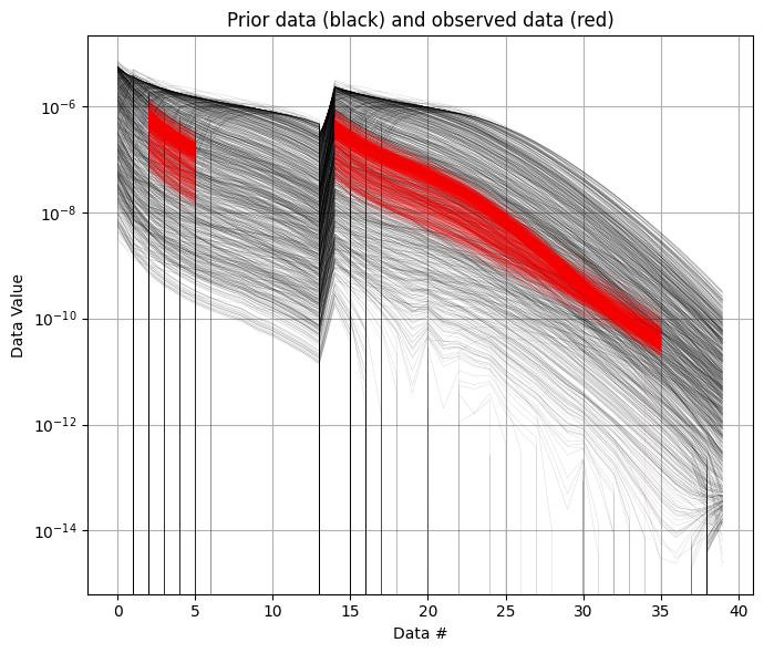
# into TWO data sets, LOW and HIGH moment.

ig.plot_data_prior(f_prior_data_h5, f_data_h5)
[5]:
True
[6]:
# Read D_obs from f_data_h5
with h5py.File(f_data_h5, 'r') as f:
D_obs = f['D1/d_obs'][:]
D_std = f['D1/d_std'][:]
# Alternatively, use the ig.load_data function
#D_obs = ig.load_data(f_data_h5, id=1, showInfo=1)['d_obs'][0]
#D_std = ig.load_data(f_data_h5, id=1, showInfo=1)['d_std'][0]
with h5py.File(f_prior_data_h5, 'r') as f:
D = f['/D1'][:]
# Alternatively, use the ig.load_prior_data function
#D = ig.load_prior_data(f_prior_data_h5)[0][0]
# Now splot the into low and high moment data sets
# The low moment data set will be the first 14 columns, and the high moment data set will be the last columns.
nd = D_obs.shape[1]
n_low = 14
n_high = nd - n_low
# set i low to 0:n_low-1
i_low = range(n_low)
i_high = range(n_low, nd)
# Split prior data
D_low = D[:,i_low]
D_high = D[:,i_high]
# Split observed data
D_obs_low = D_obs[:,i_low]
D_std_low = D_std[:,i_low]*2
D_obs_high = D_obs[:,i_high]
D_std_high = D_std[:,i_high]*2
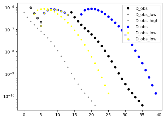
plt.semilogy(D_obs[0],'k.',markersize=10, label='D_obs')
plt.semilogy(D_obs_low[0],'.', color='gray', markersize=6, label='D_obs_low')
plt.semilogy(D_obs_high[0],'.', color='gray',markersize=4, label='D_obs_high')
plt.semilogy(D[0],'b.',markersize=10, label='D_obs')
plt.semilogy(D_low[0],'.', color='yellow', markersize=6, label='D_obs_low')
plt.semilogy(D_high[0],'.', color='yellow', markersize=6, label='D_obs_low')
plt.legend()
[6]:
<matplotlib.legend.Legend at 0x774224f1d040>
[ ]:
[7]:
f_data_dual_h5 = 'DAUGAARD_AVG_dual.h5'

useOldMethod = False
if useOldMethod:
    ig.copy_hdf5_file(f_data_h5,f_data_dual_h5)
    # Delete D1
    with h5py.File(f_data_dual_h5, 'a') as f:
        # show groups in f['']
        if 'D1' in f.keys():
            del(f['D1'])
    # Update D1 and D2
    with h5py.File(f_data_dual_h5, 'a') as f:
        # remove 'D1'
        #del f['D1']
        f.create_dataset('D1/d_obs', data=D_obs_low)
        f.create_dataset('D1/d_std', data=D_std_low)
        f['D1'].attrs['noise_model'] = 'gaussian'
        f.create_dataset('D2/d_obs', data=D_obs_high)
        f.create_dataset('D2/d_std', data=D_std_high)
        f['D2'].attrs['noise_model'] = 'gaussian'
else:
    # Alternatively, use the ig.save_data_gaussian function
    ig.copy_hdf5_file(f_data_h5,f_data_dual_h5)
    ig.save_data_gaussian(D_obs_low, D_std = D_std_low, f_data_h5 = f_data_dual_h5, id=1, showInfo=0)
    ig.save_data_gaussian(D_obs_high, D_std = D_std_high, f_data_h5 = f_data_dual_h5, id=2, showInfo=0)
Data has 11693 stations and 14 channels
Removing group DAUGAARD_AVG_dual.h5:D1
Adding group DAUGAARD_AVG_dual.h5:D1
Data has 11693 stations and 26 channels
Adding group DAUGAARD_AVG_dual.h5:D2
[8]:
f_prior_data_dual_h5 = 'PRIOR_dual.h5'
ig.copy_hdf5_file(f_prior_data_h5,f_prior_data_dual_h5)
if useOldMethod:

    with h5py.File(f_prior_data_dual_h5, 'a') as f:
        # show groups in f['']
        if 'D1' in f.keys():
            del(f['D1'])
        f.create_dataset('D1', data=D_low)
        f.create_dataset('D2', data=D_high)
else:
    # Alternatively, use the ig.save_data_gaussian function
    ig.save_prior_data(f_prior_data_dual_h5, D_low, id=1, force_delete=True)
    ig.save_prior_data(f_prior_data_dual_h5, D_high, id=2, force_delete=False)
Deleting prior data '/D1' from file: <HDF5 file "PRIOR_dual.h5" (mode r+)>
[9]:
ig.plot_data_prior(f_prior_data_dual_h5, f_data_dual_h5, id=1)
ig.plot_data_prior(f_prior_data_dual_h5, f_data_dual_h5, id=2)
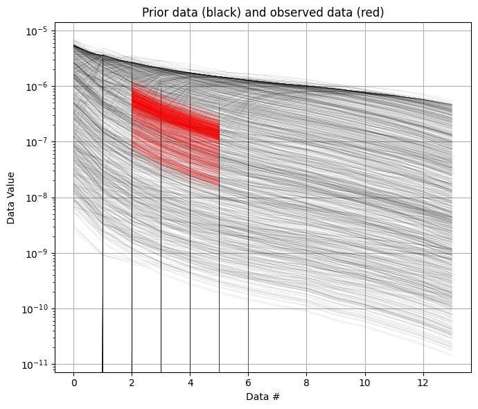
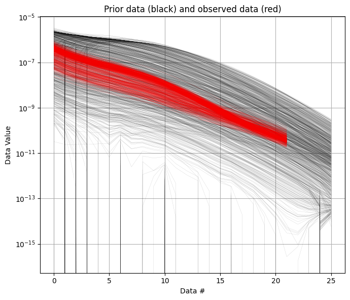
[9]:
True
Sample the posterior \(\sigma(\mathbf{m})\)
The posterior distribution is sampling using the extended rejection sampler.
[10]:
N_use = 100000 #%N
N_cpu = 8
f_post_arr = []
updatePostStat=False
showInfo = 1

import time
t_inversion = []

for itype in [0,1,2,3]:
    t_start = time.time()
    if itype == 0:
        # LOW AND HIGH MOMENT AS ONE DATA SET - THE ORIGINAL METHOD
        f_post_h5 = ig.integrate_rejection(f_prior_data_h5,
                                    f_data_h5,
                                    f_post_h5='POST_type%d.h5' % itype,
                                    N_use = N_use, Ncpu=N_cpu,
                                    showInfo=showInfo,
                                    updatePostStat=updatePostStat)
    elif itype == 1:
        # LOW MOMENT ONLY
        f_post_h5 = ig.integrate_rejection(f_prior_data_dual_h5,
                                   f_data_dual_h5,
                                   f_post_h5='POST_type%d.h5' % itype,
                                   N_use = N_use, Ncpu=N_cpu,
                                   showInfo=showInfo,
                                   updatePostStat=updatePostStat,
                                   id_use = [1])
    elif itype == 2:
        # HIGH MOMENT ONLY
        f_post_h5 = ig.integrate_rejection(f_prior_data_dual_h5,
                                   f_data_dual_h5,
                                #    f_post_h5='POST_type%d.h5' % itype,
                                   N_use = N_use, Ncpu=N_cpu,
                                   showInfo=showInfo,
                                   updatePostStat=updatePostStat,
                                   id_use = [2])
    elif itype == 3:
        # JOINT INVERSION USING BOTH LOW AND HIGH MOMENT
        f_post_h5 = ig.integrate_rejection(f_prior_data_dual_h5,
                                   f_data_dual_h5,
                                   f_post_h5='POST_type%d.h5' % itype,
                                   N_use = N_use, Ncpu=N_cpu,
                                   showInfo=showInfo,
                                   updatePostStat=updatePostStat,
                                   id_use = [1,2])

    t_inversion.append(time.time() - t_start)
    f_post_arr.append(f_post_h5)
Loading data from DAUGAARD_AVG.h5. Using data types: [1]
  - D1: id_prior=1,    gaussian, Using 11693/40 data
Loading prior data from PRIOR_CHI2_NF_3_log-uniform_N25000_TX07_20231016_2x4_RC20-33_Nh280_Nf12.h5. Using prior data ids: [1]
  - /D1:  N,nd = 25000/40
<--INTEGRATE_REJECTION-->
f_prior_h5=PRIOR_CHI2_NF_3_log-uniform_N25000_TX07_20231016_2x4_RC20-33_Nh280_Nf12.h5, f_data_h5=DAUGAARD_AVG.h5
f_post_h5=POST_type0.h5
integrate_rejection: Time= 47.0s/11693 soundings,  4.0ms/sounding, 248.8it/s. T_av=87.1, EV_av=-98.1
Loading data from DAUGAARD_AVG_dual.h5. Using data types: [1]
  - D1: id_prior=1,    gaussian, Using 11693/14 data
Loading prior data from PRIOR_dual.h5. Using prior data ids: [1]
  - /D1:  N,nd = 25000/14
<--INTEGRATE_REJECTION-->
f_prior_h5=PRIOR_dual.h5, f_data_h5=DAUGAARD_AVG_dual.h5
f_post_h5=POST_type1.h5
integrate_rejection: Time= 12.6s/11693 soundings,  1.1ms/sounding, 929.7it/s. T_av=1.0, EV_av=-6.2
Loading data from DAUGAARD_AVG_dual.h5. Using data types: [2]
  - D2: id_prior=2,    gaussian, Using 11693/26 data
Loading prior data from PRIOR_dual.h5. Using prior data ids: [2]
  - /D2:  N,nd = 25000/26
<--INTEGRATE_REJECTION-->
f_prior_h5=PRIOR_dual.h5, f_data_h5=DAUGAARD_AVG_dual.h5
f_post_h5=/mnt/space/space_au11687/PROGRAMMING/integrate_module/examples/POST_PRIOR_dual_Nu100000_aT1.h5
integrate_rejection: Time= 27.3s/11693 soundings,  2.3ms/sounding, 429.0it/s. T_av=17.4, EV_av=-24.6
Loading data from DAUGAARD_AVG_dual.h5. Using data types: [1, 2]
  - D1: id_prior=1,    gaussian, Using 11693/14 data
  - D2: id_prior=2,    gaussian, Using 11693/26 data
Loading prior data from PRIOR_dual.h5. Using prior data ids: [1, 2]
  - /D1:  N,nd = 25000/14
  - /D2:  N,nd = 25000/26
<--INTEGRATE_REJECTION-->
f_prior_h5=PRIOR_dual.h5, f_data_h5=DAUGAARD_AVG_dual.h5
f_post_h5=POST_type3.h5
integrate_rejection: Time= 37.6s/11693 soundings, 3.2ms/sounding, 311.0it/s. T_av=21.8, EV_av=-31.7
[11]:
for f_post_h5 in f_post_arr:
    ig.integrate_posterior_stats(f_post_h5)
[12]:
for f_post_h5 in f_post_arr:
    # % Plot Profiles
    ig.plot_profile(f_post_h5, i1=1000, i2=2000, im=1, hardcopy=hardcopy)
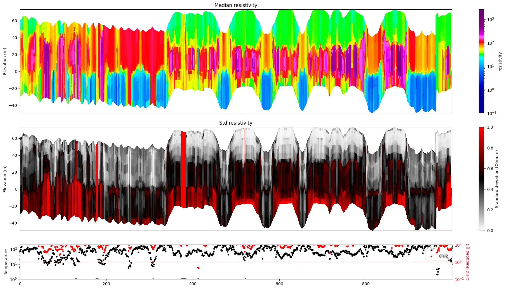
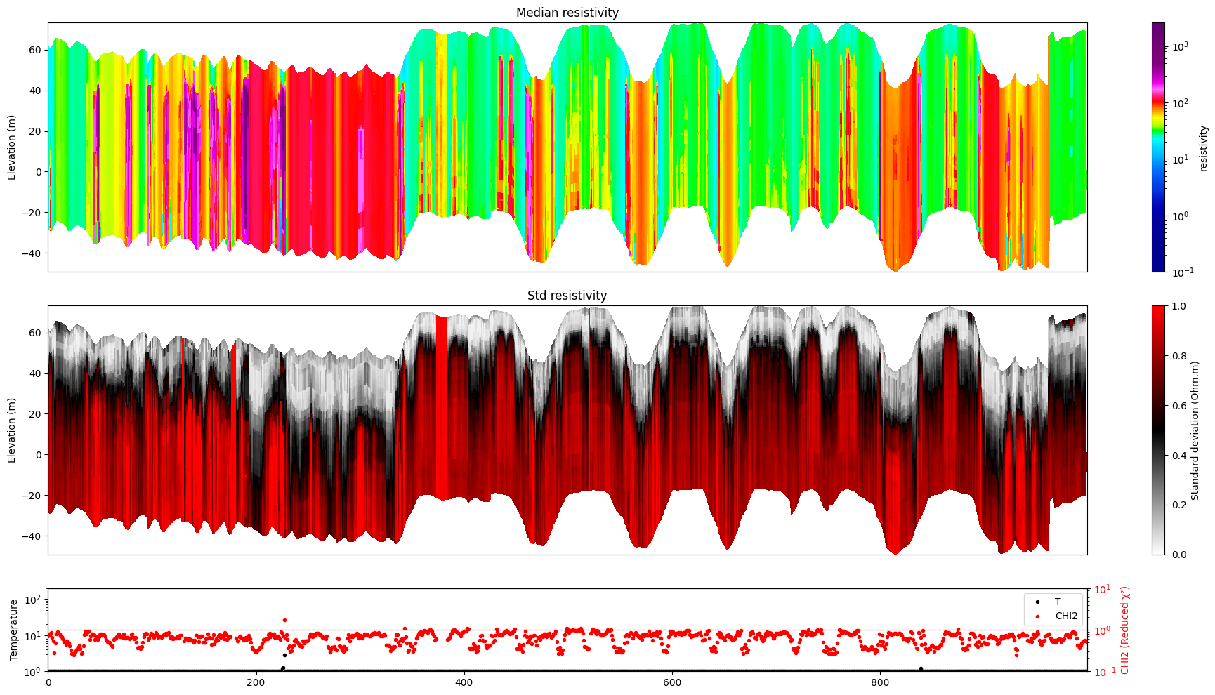
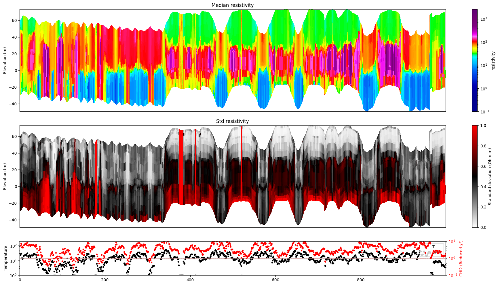
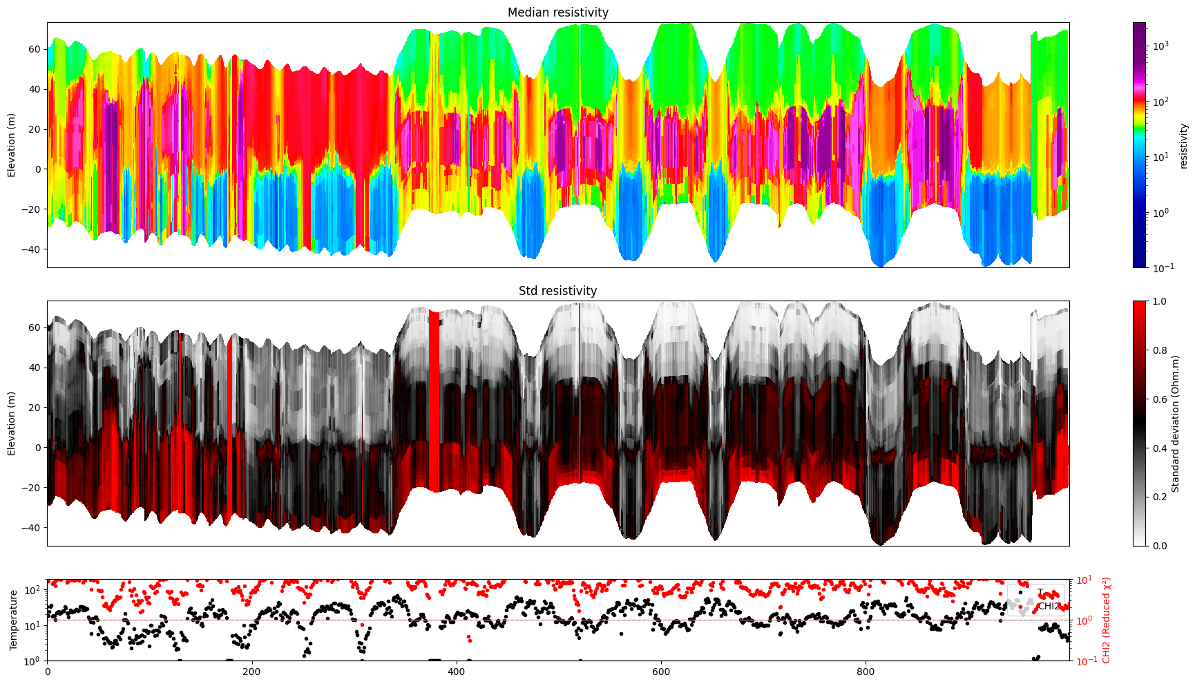
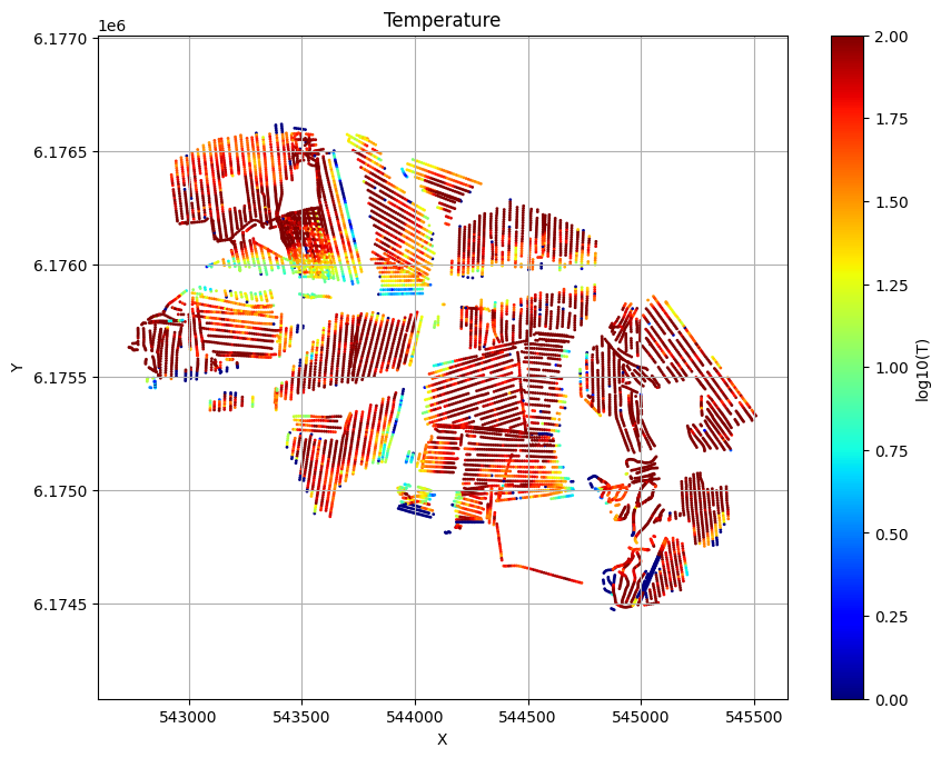
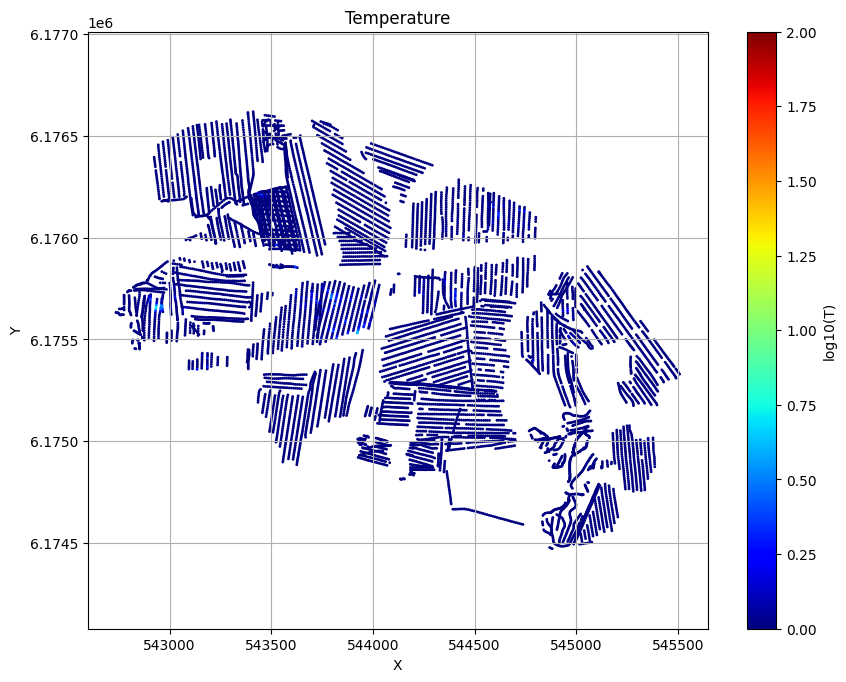
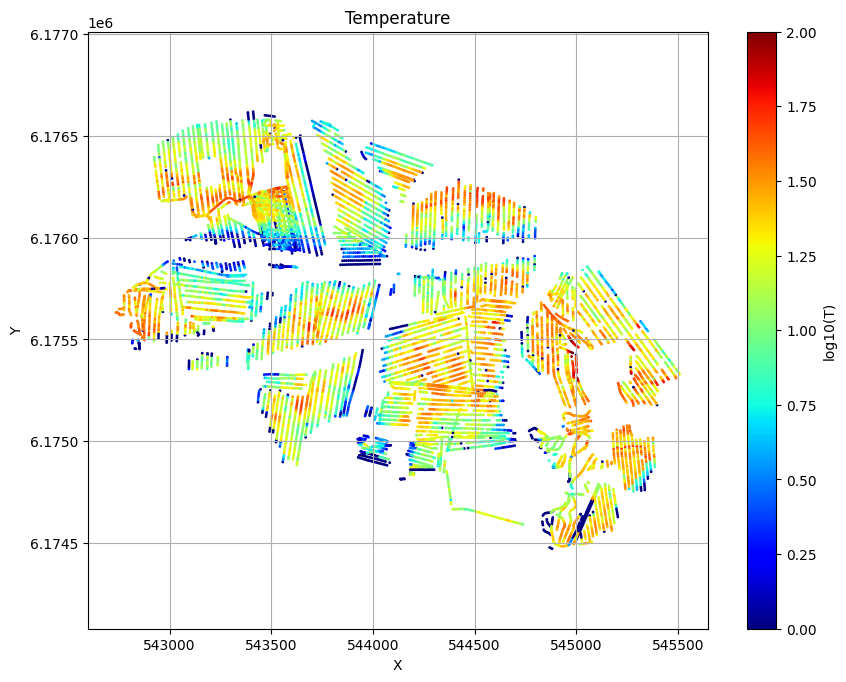
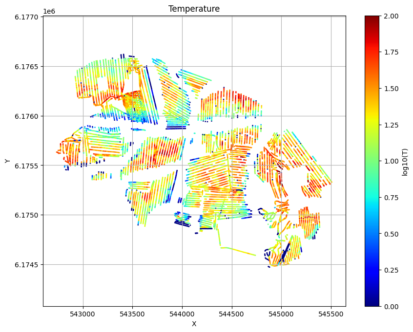
[13]:
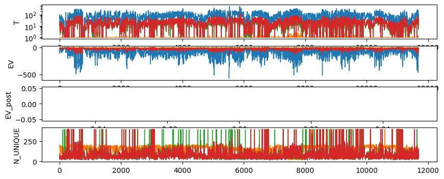
for f_post_h5 in f_post_arr:
    ig.plot_T_EV(f_post_h5, pl='T', hardcopy=hardcopy)
    plt.show()
    #ig.plot_T_EV(f_post_h5, pl='EV', hardcopy=hardcopy)
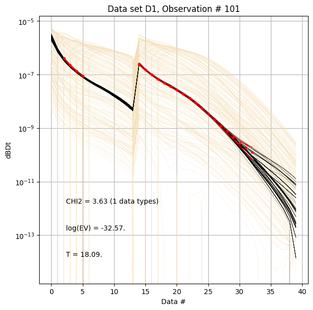
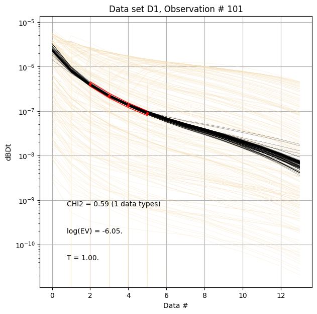
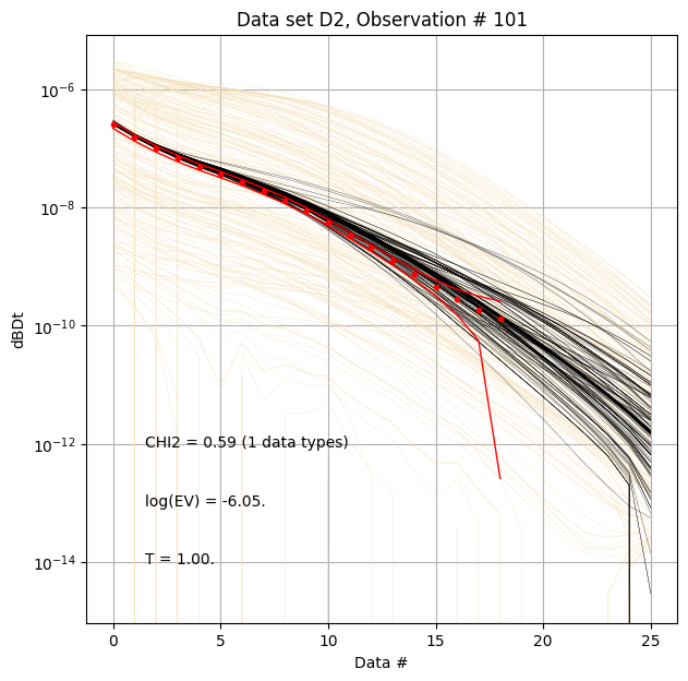
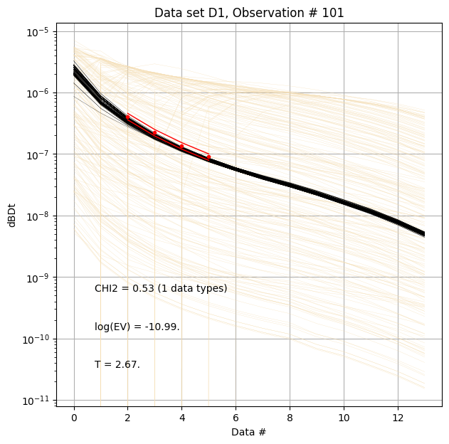
[14]:
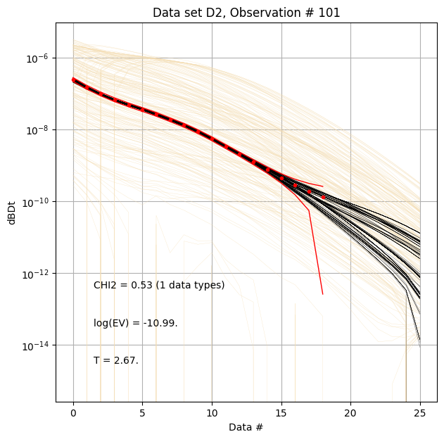
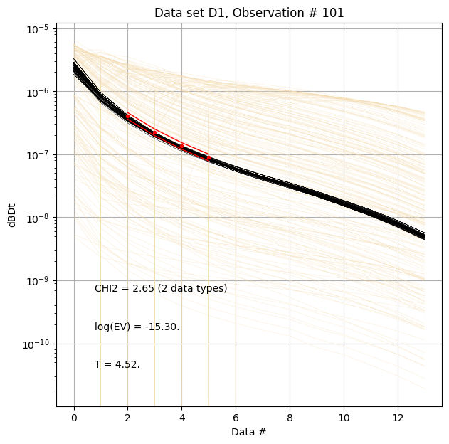
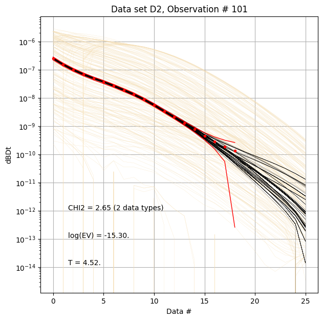
for f_post_h5 in f_post_arr:
    # % Plot prior, posterior, and observed  data
    ig.plot_data_prior_post(f_post_h5, i_plot=100, hardcopy=hardcopy)
    #ig.plot_data_prior_post(f_post_h5, i_plot=0, hardcopy=hardcopy)
[15]:
with h5py.File(f_data_h5, 'r') as f:
nobs = f['D1/d_obs'].shape[0]
ni=len(f_post_arr)
T = np.zeros((ni,nobs))
EV = np.zeros((ni,nobs))
EV_post = np.zeros((ni,nobs))
N_UNIQUE = np.zeros((ni,nobs))
i=-1
for f_post_h5 in f_post_arr:
with h5py.File(f_post_h5, 'r') as f:
i=i+1
T[i] = f['/T'][:]
EV[i] = f['/EV'][:]
N_UNIQUE[i] = f['/N_UNIQUE'][:]
EV_post[i] = f['/EV_post'][:]
fig, ax = plt.subplots(4,1,figsize=(10,4))
ax[0].semilogy(T.T,'-', linewidth=1)
ax[0].set_ylabel('T')
ax[1].plot(EV.T,'-', linewidth=1)
ax[1].set_ylabel('EV')
ax[2].plot(EV_post.T,'-', linewidth=1)
ax[2].set_ylabel('EV_post')
ax[3].plot(N_UNIQUE.T,'-', linewidth=1)
ax[3].set_ylabel('N_UNIQUE')
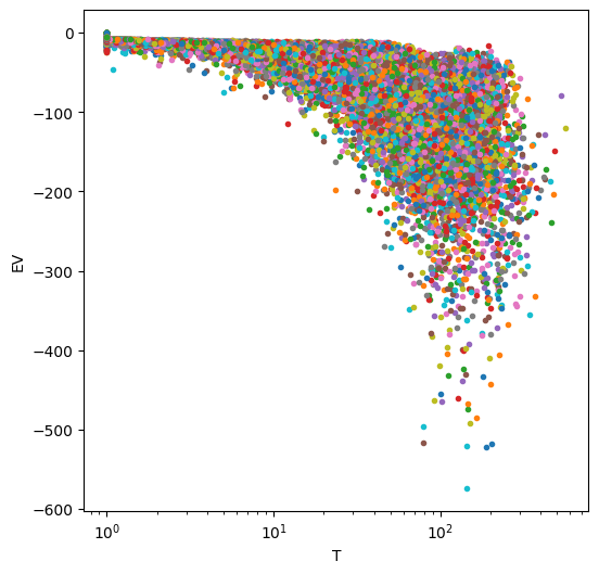
fig=plt.figure(figsize=(6,6))
plt.semilogx(T,EV,'.')
plt.xlabel('T')
plt.ylabel('EV')
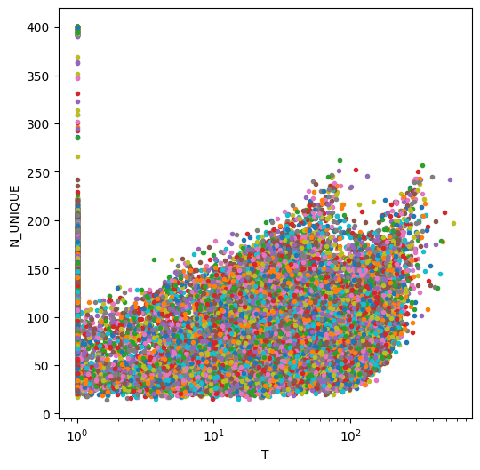
fig=plt.figure(figsize=(6,6))
plt.semilogx(T,N_UNIQUE,'.')
plt.xlabel('T')
plt.ylabel('N_UNIQUE')
[15]:
Text(0, 0.5, 'N_UNIQUE')
[16]:
#ig.post_to_csv(f_post_h5)