INTEGRATE - Demonstration of merge_prior() function
This example demonstrates how to merge multiple prior model files using the merge_prior() function. The workflow follows these main steps:
Create four different layered resistivity models:
3-layer model with low resistivity values (1-50 Ohm-m)
6-layer model with low resistivity values (1-50 Ohm-m)
3-layer model with high resistivity values (100-2000 Ohm-m)
6-layer model with high resistivity values (100-2000 Ohm-m)
Merge all four models using merge_prior() with M4 tracking source files
Generate electromagnetic forward data using DAUGAARD configuration
Perform Bayesian inversion to determine preferred model types
Analyze posterior mode of M4 parameter (discrete model selection)
[1]:
try:
    # Check if the code is running in an IPython kernel (Jupyter notebooks)
    get_ipython()
    get_ipython().run_line_magic('load_ext', 'autoreload')
    get_ipython().run_line_magic('autoreload', '2')
except:
    pass
[2]:
import integrate as ig
import numpy as np
import matplotlib.pyplot as plt
import h5py
import os

# Check if parallel computations can be performed
parallel = ig.use_parallel(showInfo=1)
hardcopy = True

print("="*60)
print("INTEGRATE - merge_prior() Function Demonstration")
print("="*60)
Notebook detected. Parallel processing is OK
============================================================
INTEGRATE - merge_prior() Function Demonstration
============================================================
1. Create four different prior models
[3]:
# Model parameters
N = 50000  # Number of samples per model
z_max = 90  # Maximum depth
f_prior_files = []

print("Creating 4 different prior models...")
print(f"- Number of samples per model: {N}")
print(f"- Maximum depth: {z_max} m")

# ### 1a. Model 1: 3-layer with low resistivity (shallow conductive layers)
print("\\n1. Creating 3-layer model with LOW resistivity (1-50 Ohm-m)...")
f_prior_3lay_low = ig.prior_model_layered(
    N=N,
    lay_dist='uniform',
    z_max=z_max,
    NLAY_min=3,
    NLAY_max=3,  # Fixed 3 layers
    RHO_dist='log-uniform',
    RHO_min=1,      # Low resistivity range
    RHO_max=50,
    f_prior_h5='PRIOR_3layer_low_rho.h5',
    showInfo=1
)
f_prior_files.append(f_prior_3lay_low)

# ### 1b. Model 2: 6-layer with low resistivity (detailed conductive structure)
print("\\n2. Creating 6-layer model with LOW resistivity (1-50 Ohm-m)...")
f_prior_6lay_low = ig.prior_model_layered(
    N=N,
    lay_dist='uniform',
    z_max=z_max,
    NLAY_min=6,
    NLAY_max=6,  # Fixed 6 layers
    RHO_dist='log-uniform',
    RHO_min=1,      # Low resistivity range
    RHO_max=50,
    f_prior_h5='PRIOR_6layer_low_rho.h5',
    showInfo=1
)
f_prior_files.append(f_prior_6lay_low)

# ### 1c. Model 3: 3-layer with high resistivity (resistive basement)
print("\\n3. Creating 3-layer model with HIGH resistivity (100-2000 Ohm-m)...")
f_prior_3lay_high = ig.prior_model_layered(
    N=N,
    lay_dist='uniform',
    z_max=z_max,
    NLAY_min=3,
    NLAY_max=3,  # Fixed 3 layers
    RHO_dist='log-uniform',
    RHO_min=100,    # High resistivity range
    RHO_max=2000,
    f_prior_h5='PRIOR_3layer_high_rho.h5',
    showInfo=1
)
f_prior_files.append(f_prior_3lay_high)

# ### 1d. Model 4: 6-layer with high resistivity (detailed resistive structure)
print("\\n4. Creating 6-layer model with HIGH resistivity (100-2000 Ohm-m)...")
f_prior_6lay_high = ig.prior_model_layered(
    N=N,
    lay_dist='uniform',
    z_max=z_max,
    NLAY_min=6,
    NLAY_max=6,  # Fixed 6 layers
    RHO_dist='log-uniform',
    RHO_min=100,    # High resistivity range
    RHO_max=2000,
    f_prior_h5='PRIOR_6layer_high_rho.h5',
    showInfo=1
)
f_prior_files.append(f_prior_6lay_high)
Creating 4 different prior models...
- Number of samples per model: 50000
- Maximum depth: 90 m
\n1. Creating 3-layer model with LOW resistivity (1-50 Ohm-m)...
prior_model_layered: Saving prior model to PRIOR_3layer_low_rho.h5
File PRIOR_3layer_low_rho.h5 does not exist.
\n2. Creating 6-layer model with LOW resistivity (1-50 Ohm-m)...
prior_model_layered: Saving prior model to PRIOR_6layer_low_rho.h5
File PRIOR_6layer_low_rho.h5 does not exist.
\n3. Creating 3-layer model with HIGH resistivity (100-2000 Ohm-m)...
prior_model_layered: Saving prior model to PRIOR_3layer_high_rho.h5
File PRIOR_3layer_high_rho.h5 does not exist.
\n4. Creating 6-layer model with HIGH resistivity (100-2000 Ohm-m)...
prior_model_layered: Saving prior model to PRIOR_6layer_high_rho.h5
File PRIOR_6layer_high_rho.h5 does not exist.
2. FORWARD response
[4]:
print("\\n" + "="*60)
print("FORWARD MODELING")
print("="*60)

# Use the DAUGAARD electromagnetic system configuration
file_gex = 'TX07_20231016_2x4_RC20-33.gex'
f_data_h5 = 'DAUGAARD_AVG.h5'

print(f"\\nGenerating electromagnetic forward data...")
print(f"- Using GEX file: {file_gex}")
print(f"- Prior files: {f_prior_files}")
print(f"- Observational data: {f_data_h5}")

f_prior_data_files = []
for i in range(len(f_prior_files)):
    f_prior = f_prior_files[i]
    print(f_prior)
    f_prior_data = ig.prior_data_gaaem(f_prior, file_gex, parallel=parallel, showInfo=0)
    f_prior_data_files.append(f_prior_data)
\n============================================================
FORWARD MODELING
============================================================
\nGenerating electromagnetic forward data...
- Using GEX file: TX07_20231016_2x4_RC20-33.gex
- Prior files: ['PRIOR_3layer_low_rho.h5', 'PRIOR_6layer_low_rho.h5', 'PRIOR_3layer_high_rho.h5', 'PRIOR_6layer_high_rho.h5']
- Observational data: DAUGAARD_AVG.h5
PRIOR_3layer_low_rho.h5
Using file_basename=TX07_20231016_2x4_RC20-33
prior_data_gaaem: Using 32 parallel threads.
prior_data_gaaem: Time= 44.4s/50000 soundings.  0.9ms/sounding, 1125.6it/s
PRIOR_6layer_low_rho.h5
Using file_basename=TX07_20231016_2x4_RC20-33
prior_data_gaaem: Using 32 parallel threads.
prior_data_gaaem: Time= 51.7s/50000 soundings.  1.0ms/sounding, 966.6it/s
PRIOR_3layer_high_rho.h5
Using file_basename=TX07_20231016_2x4_RC20-33
prior_data_gaaem: Using 32 parallel threads.
prior_data_gaaem: Time= 40.9s/50000 soundings.  0.8ms/sounding, 1221.5it/s
PRIOR_6layer_high_rho.h5
Using file_basename=TX07_20231016_2x4_RC20-33
prior_data_gaaem: Using 32 parallel threads.
prior_data_gaaem: Time= 48.6s/50000 soundings. 1.0ms/sounding, 1028.6it/s
2. Merge all four models using merge_prior()
[5]:
print("\\n" + "="*60)
print("MERGING PRIOR MODELS: %s " % (f_prior_files))
print("="*60)

# Merge all models into one
f_prior_merged = 'PRIOR_merged_4models.h5'
print(f"\\nMerging {len(f_prior_files)} prior models into: {f_prior_merged}")
print("Input files:")
for i, f in enumerate(f_prior_files):
    print(f"  {i}: {f}")
# Perform the merge model and data
f_merged = ig.merge_prior(f_prior_data_files, f_prior_merged_h5=f_prior_merged, showInfo=2)

print(f"\\nMerge completed successfully!")
print(f"Output file: {f_merged}")
\n============================================================
MERGING PRIOR MODELS: ['PRIOR_3layer_low_rho.h5', 'PRIOR_6layer_low_rho.h5', 'PRIOR_3layer_high_rho.h5', 'PRIOR_6layer_high_rho.h5']
============================================================
\nMerging 4 prior models into: PRIOR_merged_4models.h5
Input files:
  0: PRIOR_3layer_low_rho.h5
  1: PRIOR_6layer_low_rho.h5
  2: PRIOR_3layer_high_rho.h5
  3: PRIOR_6layer_high_rho.h5
Merging 4 prior files to PRIOR_merged_4models.h5
.. Processing file 1/4: PRIOR_3layer_low_rho_TX07_20231016_2x4_RC20-33_Nh280_Nf12.h5
.. Processing file 2/4: PRIOR_6layer_low_rho_TX07_20231016_2x4_RC20-33_Nh280_Nf12.h5
.. Processing file 3/4: PRIOR_3layer_high_rho_TX07_20231016_2x4_RC20-33_Nh280_Nf12.h5
.. Processing file 4/4: PRIOR_6layer_high_rho_TX07_20231016_2x4_RC20-33_Nh280_Nf12.h5
.. Concatenating arrays
.. Shuffling realizations
Shuffling 200000 realizations (seed=42 for reproducibility)
.. Writing merged file
Successfully merged 200000 samples from 4 files
Added M4 parameter tracking source file indices
\nMerge completed successfully!
Output file: PRIOR_merged_4models.h5
[ ]:
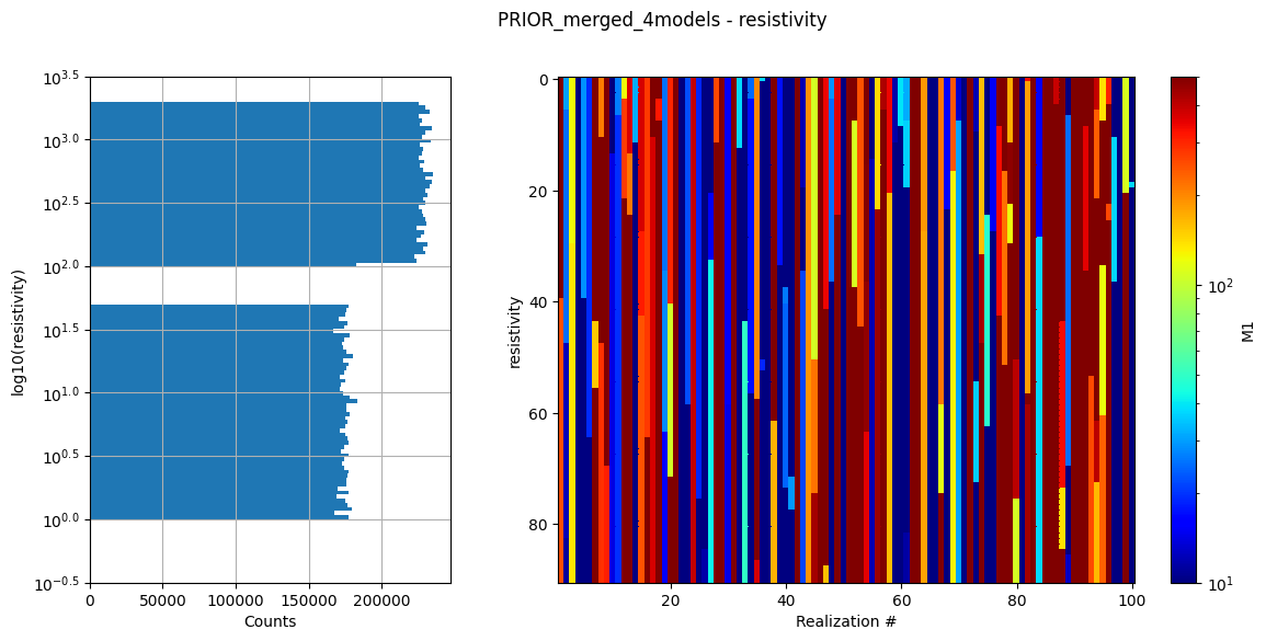
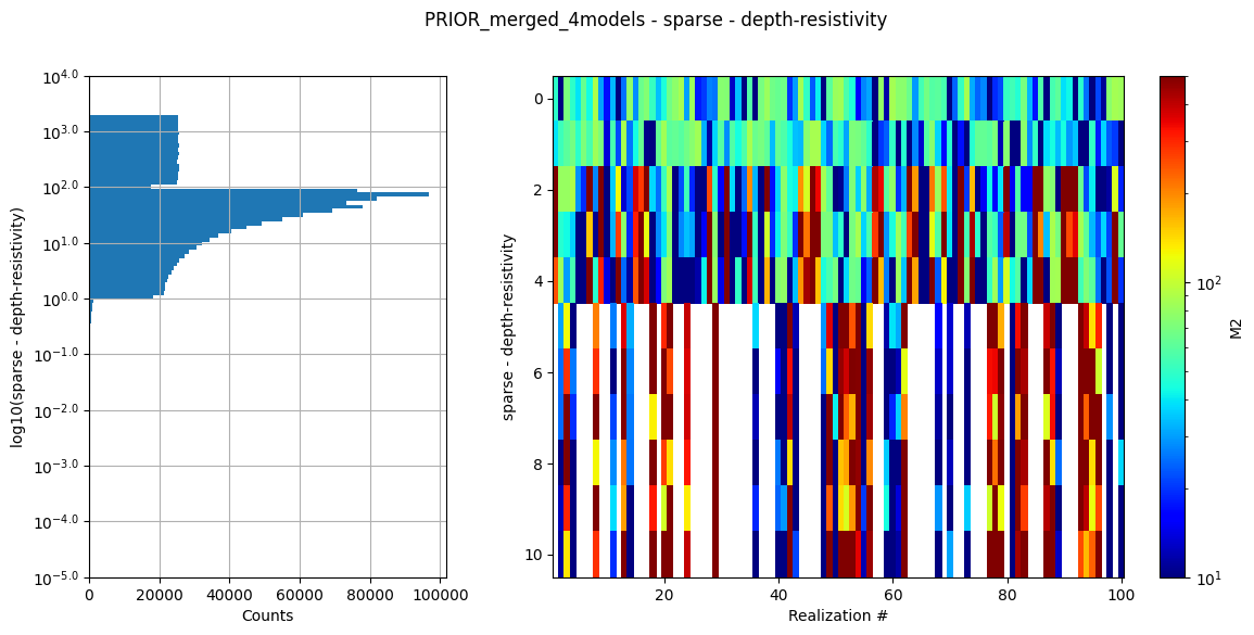
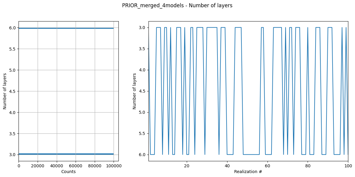
[6]:
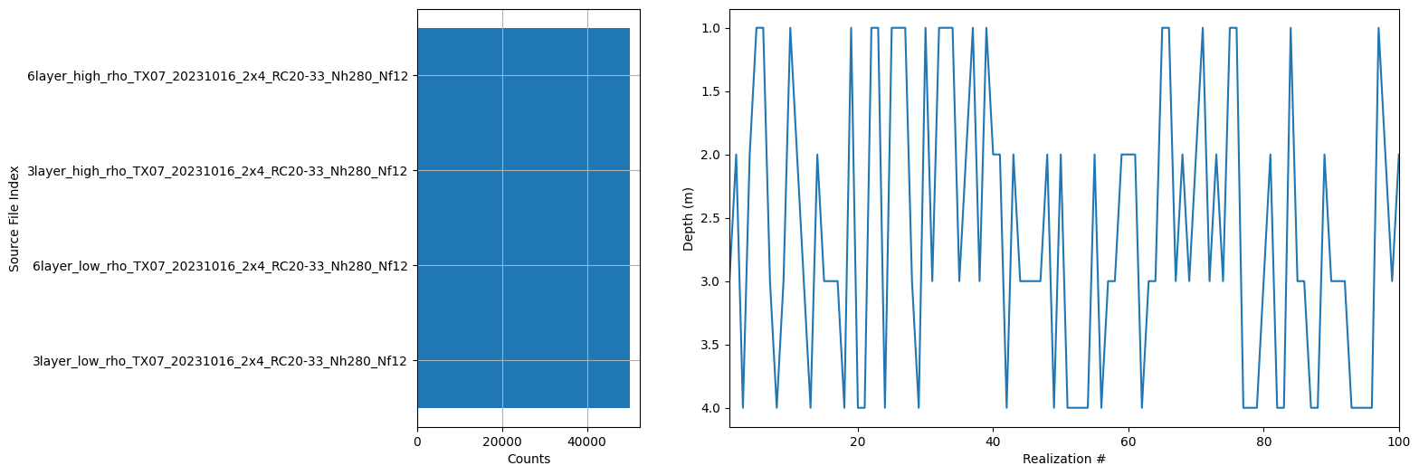
ig.integrate_update_prior_attributes(f_merged)
ig.plot_prior_stats(f_merged)
<Attributes of HDF5 object at 138727695272672>
[ ]:
5. Probabilistic inversion with integrate_rejection
[7]:
print("\\n" + "="*60)
print("PROBABILISTIC INVERSION")
print("="*60)

print(f"\\nRunning probabilistic inversion...")
print(f"- Prior data file: {f_prior_merged}")
print(f"- Observational data: {f_data_h5}")
\n============================================================
PROBABILISTIC INVERSION
============================================================
\nRunning probabilistic inversion...
- Prior data file: PRIOR_merged_4models.h5
- Observational data: DAUGAARD_AVG.h5
[8]:
# Run integrate_rejection for probabilistic inversion
f_post_h5 = ig.integrate_rejection(
    f_prior_merged,
    f_data_h5,
    f_post_h5='POST_merged_4models.h5',
    autoT=True,        # Use temperature annealing
    parallel=parallel, # Use parallel processing if available
    showInfo=1
)

print(f"\\nProbabilistic inversion completed!")
print(f"Posterior file: {f_post_h5}")
Loading data from DAUGAARD_AVG.h5. Using data types: [1]
  - D1: id_prior=1,    gaussian, Using 11693/40 data
Loading prior data from PRIOR_merged_4models.h5. Using prior data ids: [1]
  - /D1:  N,nd = 200000/40
<--INTEGRATE_REJECTION-->
f_prior_h5=PRIOR_merged_4models.h5, f_data_h5=DAUGAARD_AVG.h5
f_post_h5=POST_merged_4models.h5
integrate_rejection: Time=168.8s/11693 soundings, 14.4ms/sounding, 69.3it/s. T_av=59.2, EV_av=-367.7
Computing posterior statistics for 11693 of 11693 data points
Creating /M1/Mean in POST_merged_4models.h5
Creating /M1/Median in POST_merged_4models.h5
Creating /M1/Std in POST_merged_4models.h5
Creating /M1/LogMean in POST_merged_4models.h5
Creating /M2/Mean in POST_merged_4models.h5
Creating /M2/Median in POST_merged_4models.h5
Creating /M2/Std in POST_merged_4models.h5
Creating /M2/LogMean in POST_merged_4models.h5
Creating /M3/Mean in POST_merged_4models.h5
Creating /M3/Median in POST_merged_4models.h5
Creating /M3/Std in POST_merged_4models.h5
Creating /M3/LogMean in POST_merged_4models.h5
Creating /M4/Mode in POST_merged_4models.h5
Creating /M4/Entropy in POST_merged_4models.h5
Creating /M4/P
\nProbabilistic inversion completed!
Posterior file: POST_merged_4models.h5
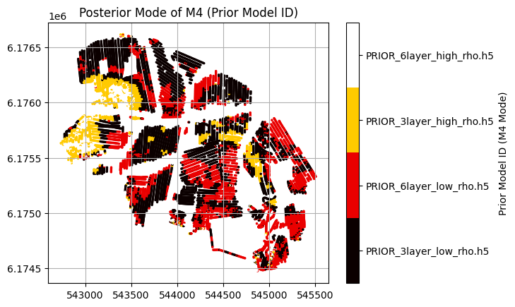
6. Analyze posterior mode of M4 parameter (prior model ID)
[9]:
print("\\n" + "="*60)
print("POSTERIOR ANALYSIS - M4 PARAMETER (PRIOR MODEL ID)")
print("="*60)

# Load posterior results and geometry
X, Y, LINE, ELEVATION = ig.get_geometry(f_data_h5)

with h5py.File(f_post_h5, 'r') as f_post:
    with h5py.File(f_merged, 'r') as f_prior:
        # Load M4 data and posterior statistics
        M4_mode = f_post['M4/Mode'][:]
        M4_entropy = f_post['M4/Entropy'][:]
        M4_P = f_post['M4/P'][:]

        # Load class names for interpretation
        class_names = [s.decode() if hasattr(s, 'decode') else s for s in f_prior['M4'].attrs['class_name']]

        print(f"\\nPosterior M4 (Prior Model ID) Analysis:")
        print(f"- Total measurement locations: {len(M4_mode)}")
        print(f"- Class names: {class_names}")

        # Count mode occurrences
        unique_modes, mode_counts = np.unique(M4_mode, return_counts=True)
        print(f"\\nPosterior mode distribution:")
        for mode, count in zip(unique_modes, mode_counts):
            percentage = (count / len(M4_mode)) * 100
            class_name = class_names[int(mode) - 1] if int(mode) <= len(class_names) else f"Class_{int(mode)}"
            print(f"  Mode {int(mode)} ({class_name}): {count} locations ({percentage:.1f}%)")
\n============================================================
POSTERIOR ANALYSIS - M4 PARAMETER (PRIOR MODEL ID)
============================================================
\nPosterior M4 (Prior Model ID) Analysis:
- Total measurement locations: 11693
- Class names: ['3layer_low_rho_TX07_20231016_2x4_RC20-33_Nh280_Nf12', '6layer_low_rho_TX07_20231016_2x4_RC20-33_Nh280_Nf12', '3layer_high_rho_TX07_20231016_2x4_RC20-33_Nh280_Nf12', '6layer_high_rho_TX07_20231016_2x4_RC20-33_Nh280_Nf12']
\nPosterior mode distribution:
  Mode 1 (3layer_low_rho_TX07_20231016_2x4_RC20-33_Nh280_Nf12): 5789 locations (49.5%)
  Mode 2 (6layer_low_rho_TX07_20231016_2x4_RC20-33_Nh280_Nf12): 3766 locations (32.2%)
  Mode 3 (3layer_high_rho_TX07_20231016_2x4_RC20-33_Nh280_Nf12): 1626 locations (13.9%)
  Mode 4 (6layer_high_rho_TX07_20231016_2x4_RC20-33_Nh280_Nf12): 512 locations (4.4%)
[10]:
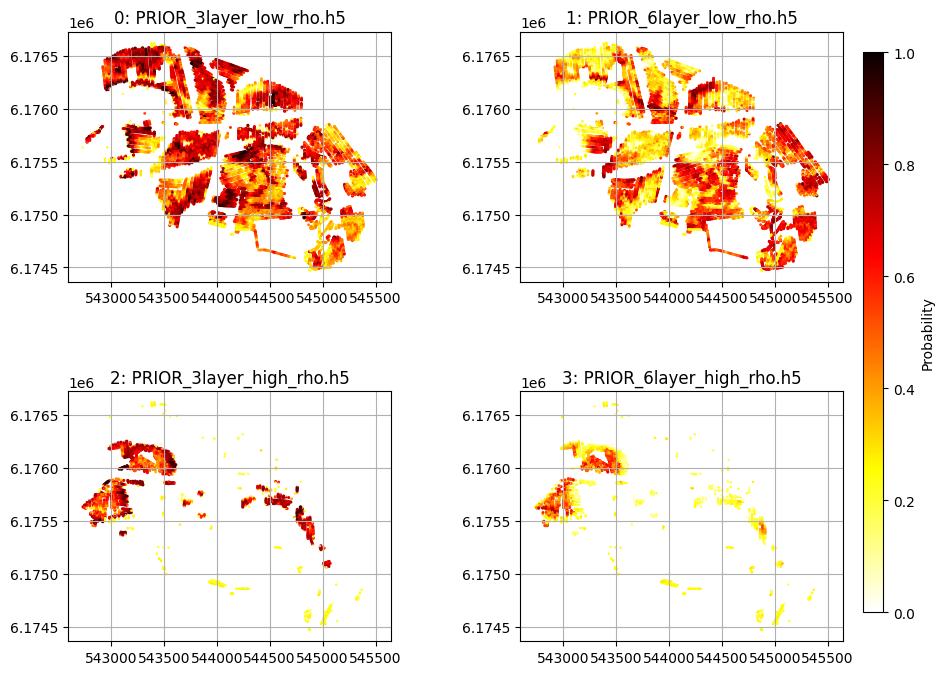
# Plot per-class probability maps (M4_P) with correct scatter args
from matplotlib import gridspec

fig = plt.figure(figsize=(10, 8))
gs = gridspec.GridSpec(2, 2, figure=fig, wspace=0.4, hspace=0.4)

for i in range(len(f_prior_files)):
    ax = fig.add_subplot(gs[i])
    sc = ax.scatter(X, Y, c=M4_P[:, i, 0], vmin=0, vmax=1, cmap='hot_r', s=2*(M4_P[:, i, 0]+.01))
    ax.set_title("%d: %s" % (i, f_prior_files[i]))
    ax.set_aspect('equal')
    plt.grid()
# Add a single colorbar for all subplots
cbar_ax = fig.add_axes([0.92, 0.15, 0.02, 0.7])  # [left, bottom, width, height]
fig.colorbar(sc, cax=cbar_ax, label='Probability')
plt.show()
[11]:
plt.figure()
# Normalize M4_entropy to control transparency (values between 0.1 and 1)
normalized_alpha = (M4_entropy - np.min(M4_entropy)) / (np.max(M4_entropy) - np.min(M4_entropy)) * 0.9 + 0.001
plt.scatter(X, Y, c=M4_mode, cmap='hot', s=2, alpha=normalized_alpha)
plt.scatter(X, Y, c=M4_mode, cmap='hot', s=2)
plt.grid()
plt.title('Posterior Mode of M4 (Prior Model ID)')
# Add a discrete colorbar with values 1, 2, 3, 4
cbar = plt.colorbar(boundaries=[0.5, 1.5, 2.5, 3.5, 4.5], ticks=[1, 2, 3, 4])
cbar.set_ticklabels(['Class 1', 'Class 2', 'Class 3', 'Class 4'])
cbar.set_ticklabels(f_prior_files)
cbar.set_label('Prior Model ID (M4 Mode)')