Daugaard Case Study with three lithology-resistivity prior models.
This notebook contains an example of inverison of the DAUGAARD tTEM data using three different lithology-resistivity prior models
[1]:
try:
    # Check if the code is running in an IPython kernel (which includes Jupyter notebooks)
    get_ipython()
    # If the above line doesn't raise an error, it means we are in a Jupyter environment
    # Execute the magic commands using IPython's run_line_magic function
    get_ipython().run_line_magic('load_ext', 'autoreload')
    get_ipython().run_line_magic('autoreload', '2')
except:
    # If get_ipython() raises an error, we are not in a Jupyter environment
    # # # # # # #%load_ext autoreload
    # # # # # # #%autoreload 2
    pass

import integrate as ig
import numpy as np
import os
import matplotlib.pyplot as plt
import h5py

from integrate.integrate_io import copy_prior
hardcopy=True
Download the data DAUGAARD data including non-trivial prior data realizations
[2]:
files = ig.get_case_data(case='DAUGAARD') # Load only data
#files = ig.get_case_data(case='DAUGAARD', loadType='prior') # Load data and prior realizations
#files = ig.get_case_data(case='DAUGAARD', loadType='prior_data') # Load data and prior+data realizations
files = ig.get_case_data(case='DAUGAARD', loadType='post') # # Load data and posterior realizations
#files = ig.get_case_data(case='DAUGAARD', loadAll=True) # All of the above
f_data_h5 = files[0]
file_gex= ig.get_gex_file_from_data(f_data_h5)
# check that file_gex exists
if not os.path.isfile(file_gex):
    print("file_gex=%s does not exist in the current folder." % file_gex)

print('Using hdf5 data file %s with gex file %s' % (f_data_h5,file_gex))
Getting data for case: DAUGAARD
--> Got data for case: DAUGAARD
Getting data for case: DAUGAARD
Downloading prior_detailed_general_N2000000_dmax90_TX07_20231016_2x4_RC20-33_Nh280_Nf12.h5
Downloaded prior_detailed_general_N2000000_dmax90_TX07_20231016_2x4_RC20-33_Nh280_Nf12.h5
Downloading prior_detailed_invalleys_N2000000_dmax90_TX07_20231016_2x4_RC20-33_Nh280_Nf12.h5
Downloaded prior_detailed_invalleys_N2000000_dmax90_TX07_20231016_2x4_RC20-33_Nh280_Nf12.h5
Downloading prior_detailed_outvalleys_N2000000_dmax90_TX07_20231016_2x4_RC20-33_Nh280_Nf12.h5
Downloaded prior_detailed_outvalleys_N2000000_dmax90_TX07_20231016_2x4_RC20-33_Nh280_Nf12.h5
Downloading daugaard_valley_new_N1000000_dmax90_TX07_20231016_2x4_RC20-33_Nh280_Nf12.h5
Downloaded daugaard_valley_new_N1000000_dmax90_TX07_20231016_2x4_RC20-33_Nh280_Nf12.h5
Downloading daugaard_standard_new_N1000000_dmax90_TX07_20231016_2x4_RC20-33_Nh280_Nf12.h5
Downloaded daugaard_standard_new_N1000000_dmax90_TX07_20231016_2x4_RC20-33_Nh280_Nf12.h5
Downloading POST_DAUGAARD_AVG_prior_detailed_general_N2000000_dmax90_TX07_20231016_2x4_RC20-33_Nh280_Nf12_Nu2000000_aT1.h5
Downloaded POST_DAUGAARD_AVG_prior_detailed_general_N2000000_dmax90_TX07_20231016_2x4_RC20-33_Nh280_Nf12_Nu2000000_aT1.h5
--> Got data for case: DAUGAARD
Using hdf5 data file DAUGAARD_AVG.h5 with gex file TX07_20231016_2x4_RC20-33.gex
[3]:
inflateNoise = 3
if inflateNoise != 1:
    gf=inflateNoise
    print("="*60)
    print("Increasing noise level (std) by a factor of %d" % gf)
    print("="*60)
    D = ig.load_data(f_data_h5)
    D_obs = D['d_obs'][0]
    D_std = D['d_std'][0]*gf
    f_data_old_h5 = f_data_h5
    f_data_h5 = 'DAUGAARD_AVG_gf%g.h5' % (gf)
    ig.copy_hdf5_file(f_data_old_h5, f_data_h5)
    ig.save_data_gaussian(D_obs, D_std=D_std, f_data_h5=f_data_h5, file_gex=file_gex)

    #ig.plot_data(f_data_old_h5)
    #ig.plot_data(f_data_h5)
============================================================
Increasing noise level (std) by a factor of 3
============================================================
Loading data from DAUGAARD_AVG.h5. Using data types: [1]
  - D1: id_prior=1,    gaussian, Using 11693/40 data
Data has 11693 stations and 40 channels
Removing group DAUGAARD_AVG_gf3.h5:D1
Adding group DAUGAARD_AVG_gf3.h5:D1
Compute prior data from prior model if they do not already exist
[4]:
# A1. CONSTRUCT PRIOR MODEL OR USE EXISTING
f_prior_h5_list = []
f_prior_h5_list.append('daugaard_valley_new_N1000000_dmax90_TX07_20231016_2x4_RC20-33_Nh280_Nf12.h5')
f_prior_h5_list.append('daugaard_standard_new_N1000000_dmax90_TX07_20231016_2x4_RC20-33_Nh280_Nf12.h5')
[5]:
# read f_prior_h5, and split it itp two priors with half the data in each
# first use ig.load_prior_data() and ig.save_prior_data()
useSubset = True
if useSubset:
    f_prior_h5 = f_prior_h5_list[0]
    # This can probably be done with more elegance!
    D, M, idx = ig.load_prior(f_prior_h5)
    Nd = D[0].shape[0]
    nsubsets = 2
    f_prior_h5_list = []
    Nd_sub = int(np.ceil(Nd/2))
    for i in range(nsubsets):
        # idx should go from i*Nd_sub to (i+1)*Nd_sub, unless in the last iteration
        # from i*Nd_sub to Nd
        idx = np.arange(i*Nd_sub, Nd) if i == nsubsets - 1 else np.arange(i*Nd_sub, (i+1)*Nd_sub)

        f_prior_data_h5 = 'prior_data_%02d_%d_%d.h5' % (i+1,idx[0],idx[-1])

        ig.copy_prior(f_prior_h5, f_prior_data_h5, idx=idx)
        f_prior_h5_list.append(f_prior_data_h5)
Loading prior data from daugaard_valley_new_N1000000_dmax90_TX07_20231016_2x4_RC20-33_Nh280_Nf12.h5. Using prior data ids: []
  - /D1:  N,nd = 1000000/40
[6]:
# Go through f_prior_data_h5_list. If the file does not exist the compute, it by runinng ig.prior_data_gaaem
f_prior_data_h5_list = []
for i in range(len(f_prior_h5_list)):
f_prior_h5= f_prior_h5_list[i]
#ig.integrate_update_prior_attributes(f_prior_h5)
# check if f_prior_h5 as a datasets called '/D1'
with h5py.File(f_prior_h5, 'r') as f:
if '/D1' not in f:
#print('Dataset /D1 not found in %s' % f_prior_h5)
print('Prior data file %s does not exist. Computing it.' % f_prior_h5)
# Compute prior data
f_prior_data_h5 = ig.prior_data_gaaem(f_prior_h5, file_gex, N=N_use)
f_prior_data_h5_list.append(f_prior_data_h5)
else:
print('Dataset /D1 found in %s' % f_prior_h5)
f_prior_data_h5_list.append(f_prior_h5)
print('Using existing prior data file %s' % f_prior_h5)
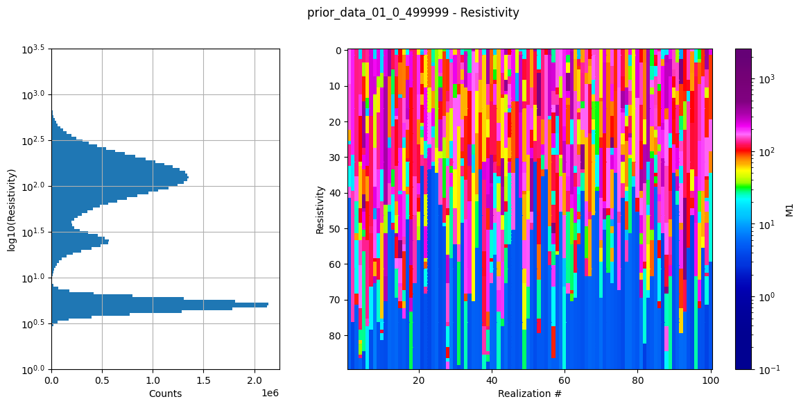
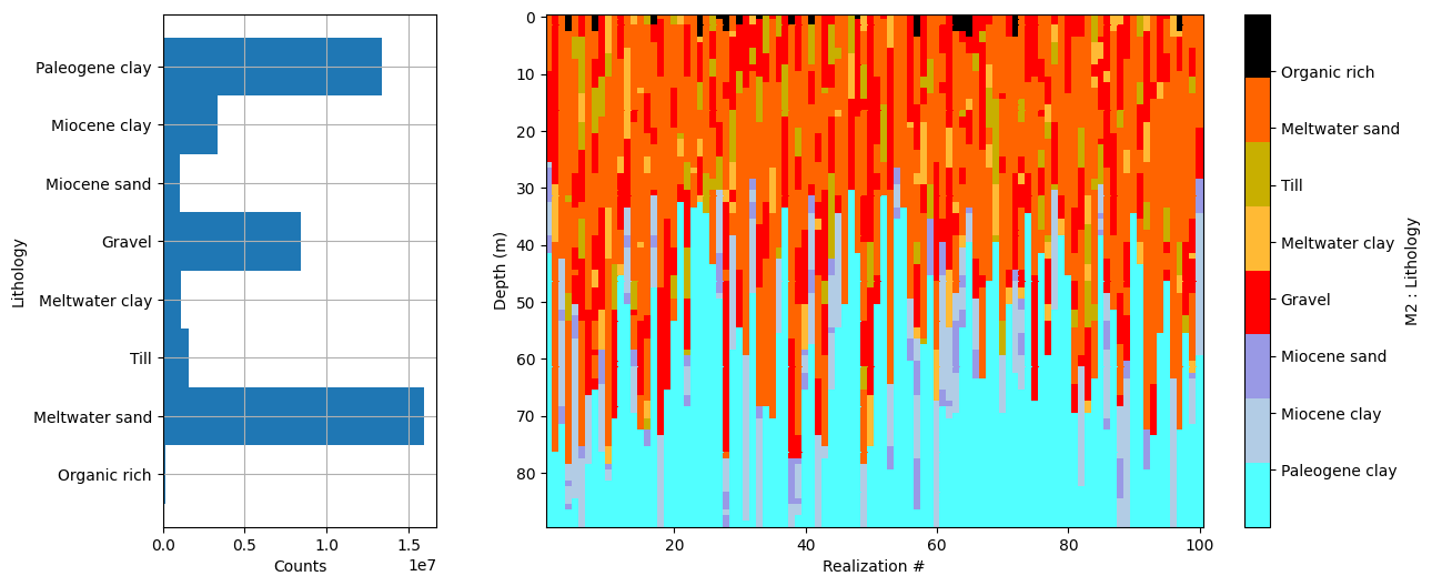
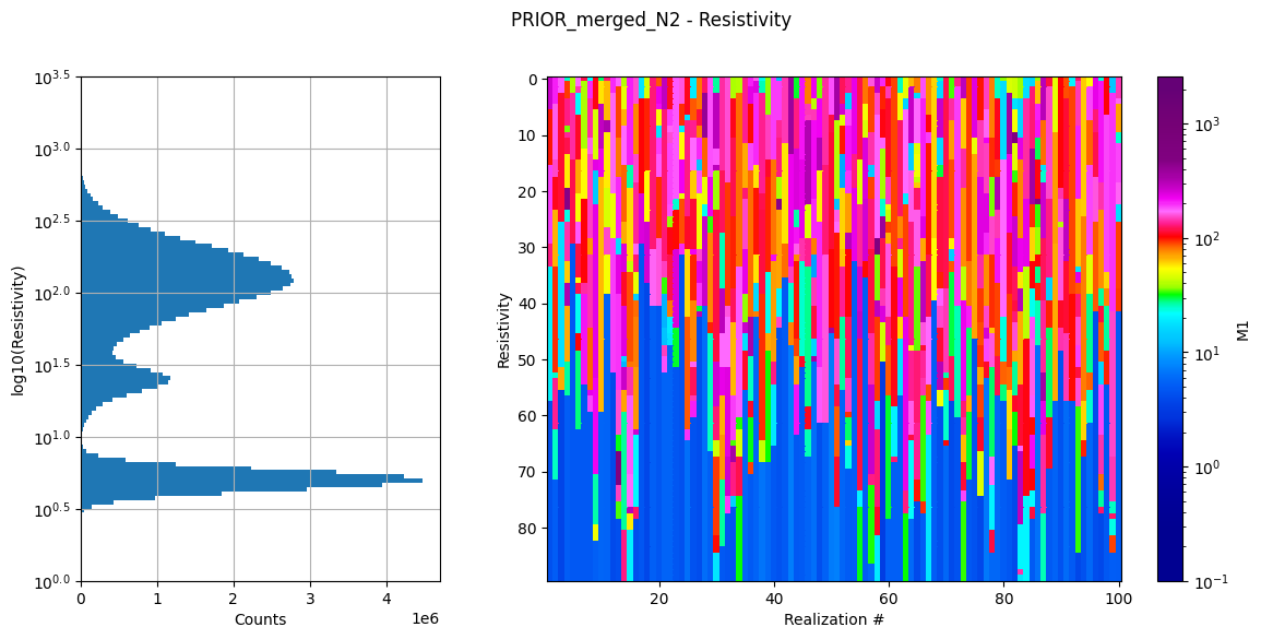
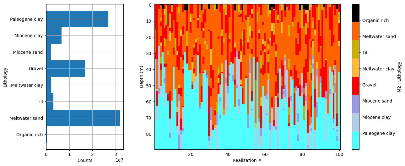
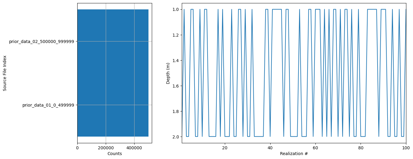
ig.plot_prior_stats(f_prior_h5)
Dataset /D1 found in prior_data_01_0_499999.h5
Using existing prior data file prior_data_01_0_499999.h5
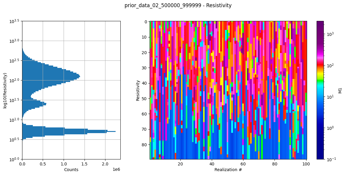
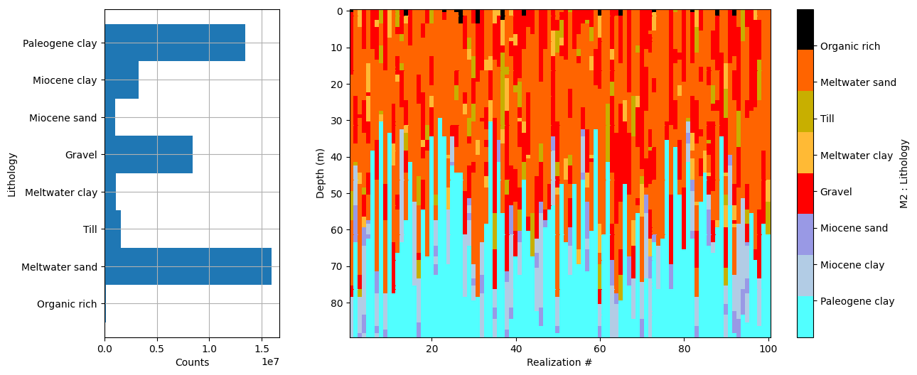
Dataset /D1 found in prior_data_02_500000_999999.h5
Using existing prior data file prior_data_02_500000_999999.h5
[7]:
# Set random seed
np.random.seed(42)
[8]:
f_post_h5_list = []

N_use = 1000
N_use = 10000
N_use = 100000
#N_use = 200000
N_use = 1000000

autoT=True
T_base = 1

txt = 'N%d_autoT%d_Tbase%g_useSub%d_inflateNoise%d' % (N_use, autoT, T_base,useSubset,inflateNoise)

for f_prior_data_h5 in f_prior_data_h5_list:
    print('Using prior model file %s' % f_prior_data_h5)

    #f_prior_data_h5 = 'gotaelv2_N1000000_fraastad_ttem_Nh280_Nf12.h5'
    updatePostStat =True


    # extract filename without extension from f_prior_data_h5
    fileparts = os.path.splitext(f_prior_data_h5)
    f_post_h5 = 'post_%s_%s.h5' % (fileparts[0],txt)


    f_post_h5 = ig.integrate_rejection(f_prior_data_h5, f_data_h5,
                                       N_use = N_use,
                                       parallel=1,
                                       T_base = T_base,
                                       autoT=autoT,
                                       updatePostStat=updatePostStat,
                                       f_post_h5=f_post_h5)
    f_post_h5_list.append(f_post_h5)
Using prior model file prior_data_01_0_499999.h5
integrate_rejection: Time=1122.1s/11693 soundings, 96.0ms/sounding, 10.4it/s. T_av=1.8, EV_av=-13.3
Using prior model file prior_data_02_500000_999999.h5
integrate_rejection: Time=891.9s/11693 soundings, 76.3ms/sounding, 13.1it/s. T_av=1.8, EV_av=-13.2
[9]:
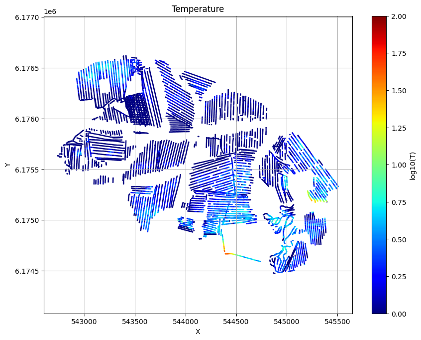
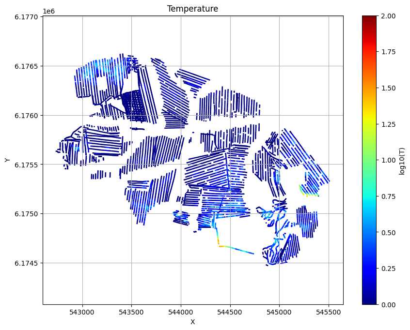
for f_post_h5 in f_post_h5_list:
    ig.plot_T_EV(f_post_h5, pl='T', hardcopy=hardcopy)
    plt.show()

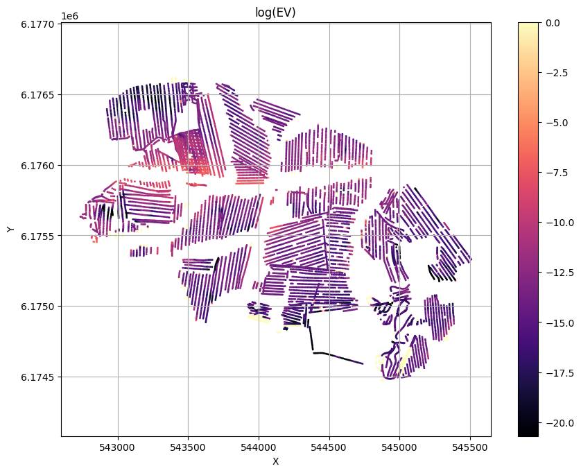
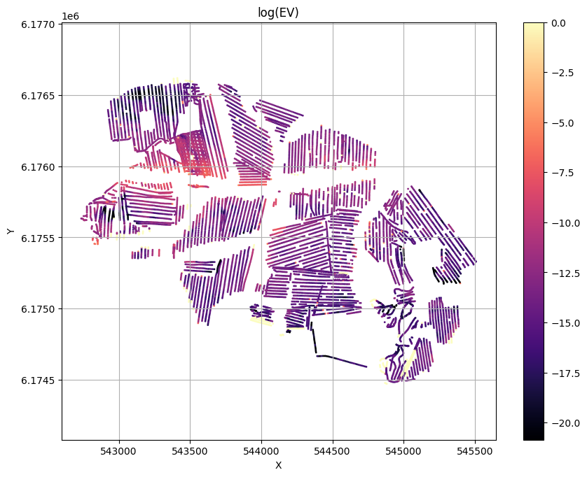
[10]:
for f_post_h5 in f_post_h5_list:
    ig.plot_T_EV(f_post_h5, pl='EV',hardcopy=hardcopy)
    plt.show()
[11]:
plotPro = False
if plotPro:
    for f_post_h5 in f_post_h5_list:
        #% Posterior analysis
        # Plot the Temperature used for inversion
        #ig.plot_T_EV(f_post_h5, pl='T')
        #ig.plot_T_EV(f_post_h5, pl='EV', hardcopy=hardcopy)
        #plt.show()

        #ig.plot_T_EV(f_post_h5, pl='ND')

        #% Plot Profiles
        ig.plot_profile(f_post_h5, i1=0, i2=2000, cmap='jet', hardcopy=hardcopy)
        plt.show()
        #% Export to CSV
        #ig.post_to_csv(f_post_h5)
        #plt.show()
[12]:
X, Y, LINE, ELEVATION = ig.get_geometry(f_data_h5)

nd=len(X)
nev=len(f_post_h5_list)

EV_mul = np.zeros((nev,nd))

iev = -1
for f_post_h5 in f_post_h5_list:
    iev += 1
    # Read '/EV' from f_post_h5
    with h5py.File(f_post_h5, 'r') as f_post:
        print(f_post_h5)
        #EV=(f_post['/EV'][:])
        EV_mul[iev]=(f_post['/EV'][:])

#% Normalize EV

EV_P = 0*EV_mul
E_max = np.max(EV_mul, axis=0)

for iev in range(nev):
    EV_P[iev] = np.exp(EV_mul[iev]-E_max)

# Use annealing to flaten prob
T_EV = 10
EV_P = EV_P**(1/T_EV)

EV_P_sum = np.sum(EV_P,axis=0)
for iev in range(nev):
    EV_P[iev] = EV_P[iev]/EV_P_sum
post_prior_data_01_0_499999_N1000000_autoT1_Tbase1_useSub1_inflateNoise3.h5
post_prior_data_02_500000_999999_N1000000_autoT1_Tbase1_useSub1_inflateNoise3.h5
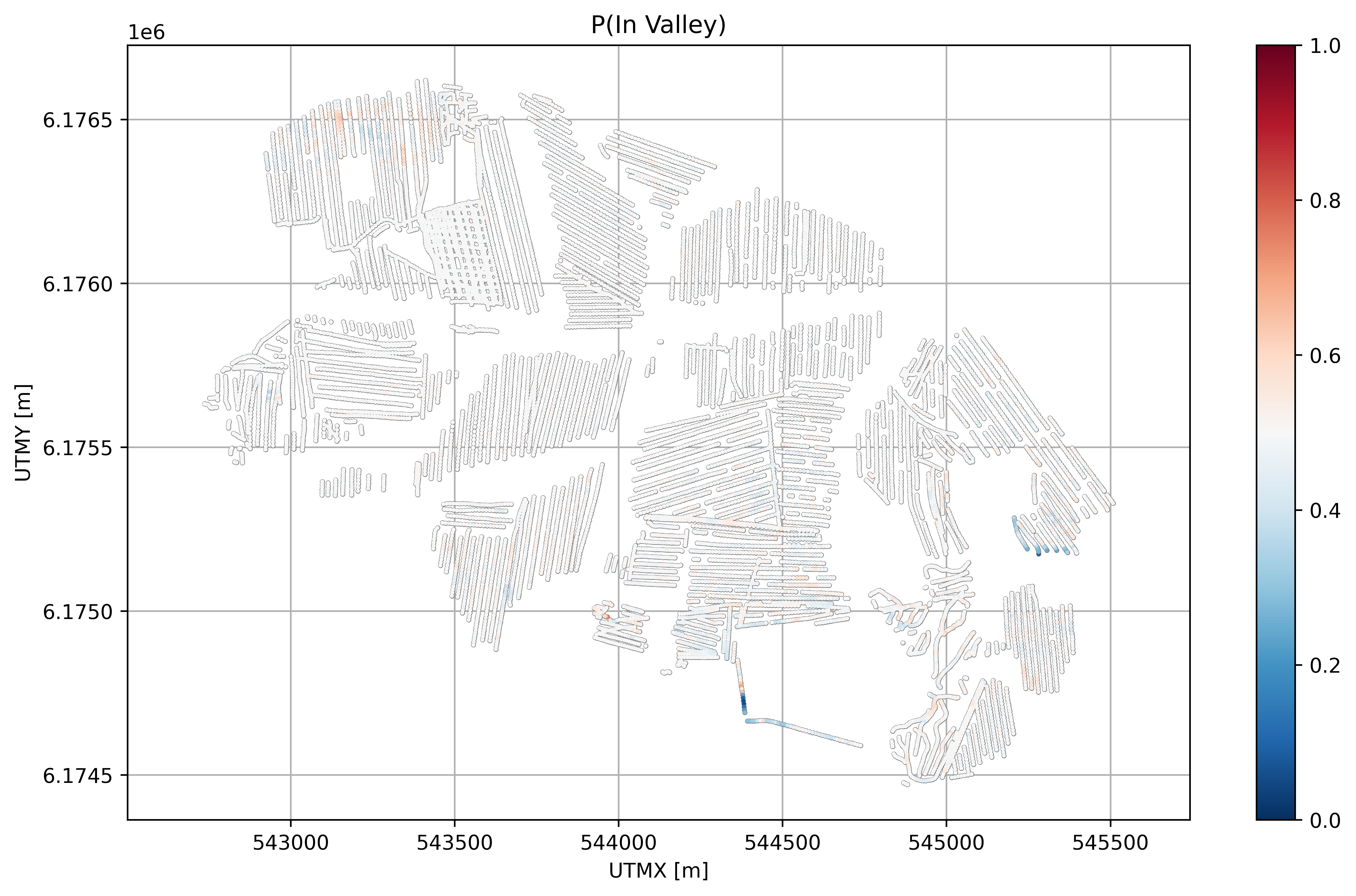
[13]:
plt.figure(figsize=(10,6), dpi=600)
plt.subplot(1,1,1)
plt.plot(X, Y, '.', markersize=3, color='gray')
plt.scatter(X, Y, c=EV_P[0], cmap='RdBu_r', s=1, vmin=0, vmax=1, zorder=2)
plt.tight_layout()
plt.axis('equal')
plt.colorbar()
plt.title('P(In Valley)')
plt.xlabel('UTMX [m]')
plt.ylabel('UTMY [m]')
plt.grid()
plt.savefig('%s_Pin.png' % (txt), dpi=600)
plt.show()
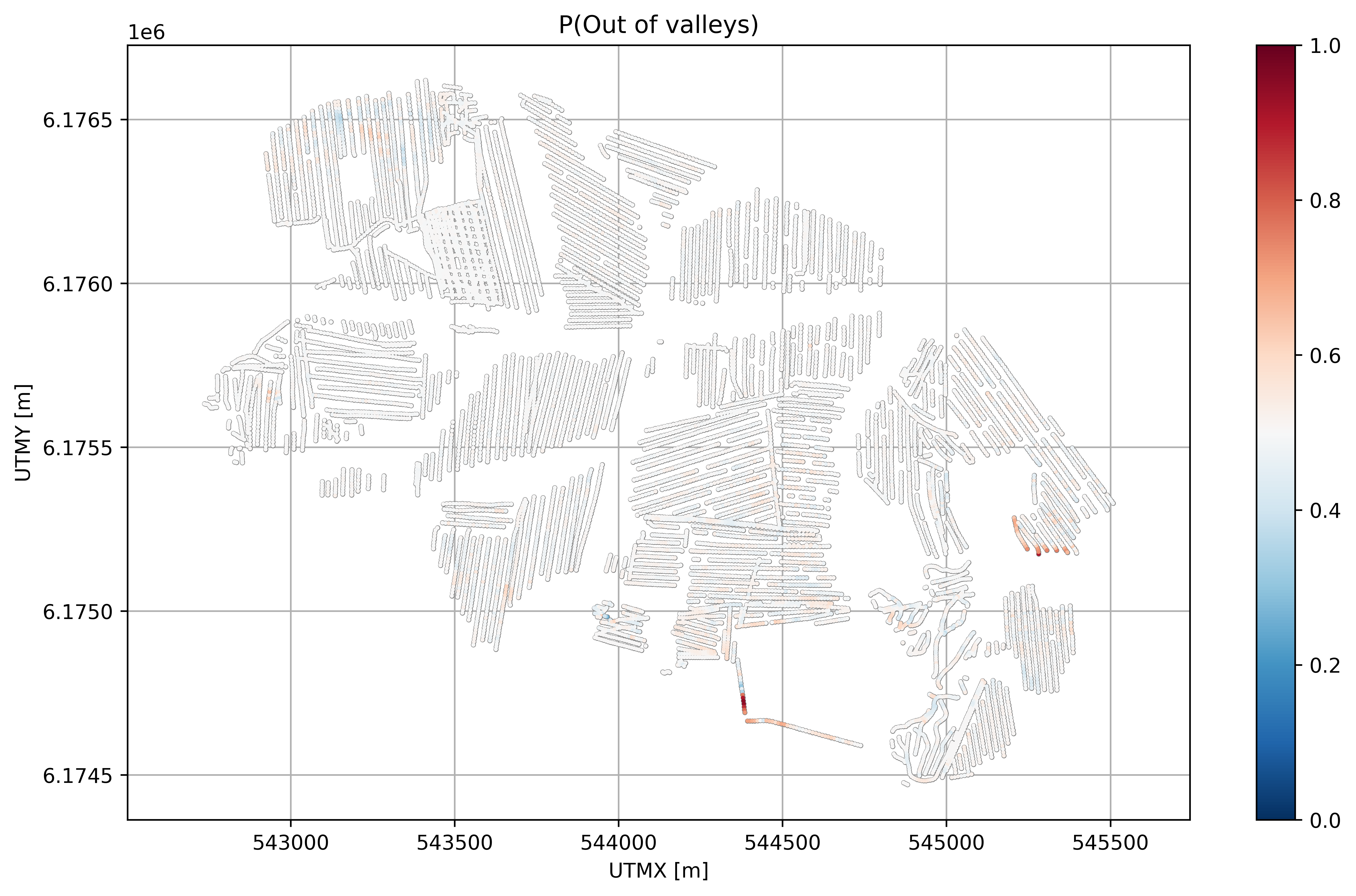
[14]:
plt.figure(figsize=(10,6), dpi=600)
plt.subplot(1,1,1)
plt.plot(X, Y, '.', markersize=3, color='gray')
plt.scatter(X, Y, c=EV_P[1], cmap='RdBu_r', s=1, vmin=0, vmax=1, zorder=2)
plt.tight_layout()
plt.axis('equal')
plt.colorbar()
plt.grid()
plt.title('P(Out of valleys)')
plt.xlabel('UTMX [m]')
plt.ylabel('UTMY [m]')
plt.savefig('%s_Pout.png' % (txt), dpi=600)
plt.show()
[15]:
plTest=False
if plTest:
    import matplotlib.colors as mcolors
    import matplotlib.pyplot as plt
    import numpy as np

    # Create a discrete two-color colormap
    colors = ['black', '#0173B2']  # Black and blue - colorblind friendly
    colors = ['red', 'blue']  # Red and yellow
    cmap = mcolors.ListedColormap(colors)

    plt.figure(figsize=(10,6), dpi=600)
    # Get the index of the highest value in each column in EV_P_sum
    EV_mode = np.argmax(EV_P, axis=0)
    EV_P_max = np.max(EV_P, axis=0)
    psize = (EV_P_max-0.5)*4+0.001
    plt.subplot(1,1,1)
    plt.plot(X, Y, 'w.', markersize=4, color='lightgray', zorder=1)
    plt.scatter(X, Y, c=EV_mode, cmap=cmap, s=psize, zorder=2)
    plt.axis('equal')
    plt.grid()
    plt.tight_layout()
    #cbar = plt.colorbar(ticks=[0, 1])
    cbar = plt.colorbar(ticks=[0.25, 0.75])
    cbar.set_ticklabels(['In', 'Out'])
    plt.xlabel('UTMX [m]')
    plt.ylabel('UTMY [m]')

    plt.savefig('DAUGAARD_N%07d_EV_mode.png' % (N_use), dpi=600)
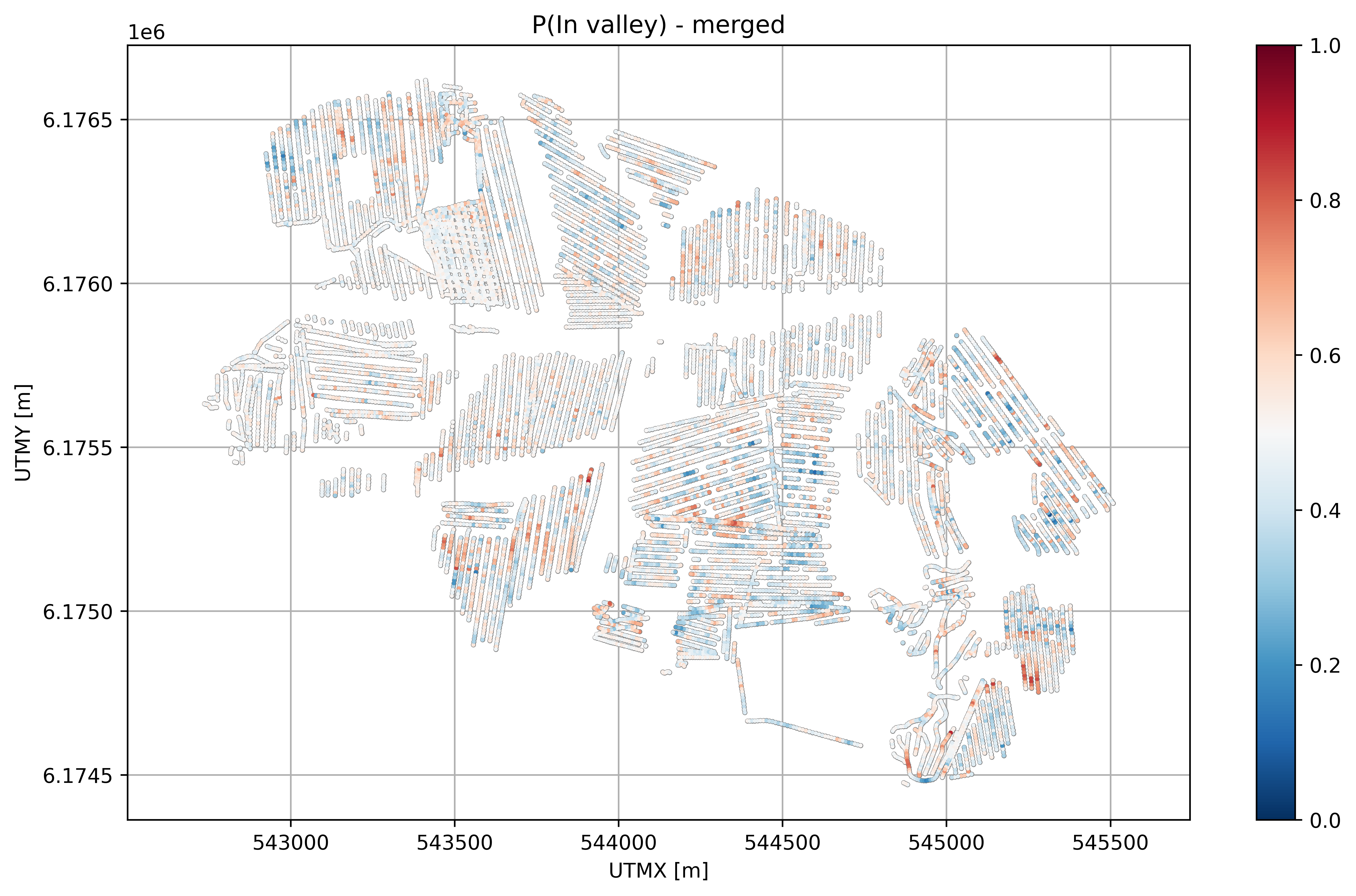
Combine the two priors and invert with them as one prior
As an alternative to using the evidence to compute the posterior hypothesis probability, two prior realizations from both priors can be combined into realizations of a single prior. This combined prior has an extra parameter ‘/M3’ in this case, which represents the ID of the original hypothesis or prior model used.
[16]:
# Merge the prior models and data
f_prior_data_h5_merged = ig.merge_prior(f_prior_data_h5_list)
ig.integrate_update_prior_attributes(f_prior_data_h5_merged)
ig.plot_prior_stats(f_prior_data_h5_merged)
[17]:
#N_use = 10000
#autoT = False
#T_base = 10

N_use_merged = 2*N_use

# Sample the posterior
#f_prior_data_h5 = 'gotaelv2_N1000000_fraastad_ttem_Nh280_Nf12.h5'
updatePostStat =True

txt_merged = 'N%d_autoT%d_Tbase%g_useSub%d_inflateNoise%d' % (N_use_merged, autoT, T_base,useSubset,inflateNoise)
fileparts = os.path.splitext(f_prior_data_h5_merged)
f_post_h5_merged = 'post_%s_%s.h5' % (fileparts[0],txt_merged)

f_post_h5_merged = ig.integrate_rejection(f_prior_data_h5_merged, f_data_h5,
                            N_use = N_use_merged,
                            parallel=1,
                            T_base = T_base,
                            autoT=autoT,
                            updatePostStat=updatePostStat,
                            showInfo=1, f_post_h5=f_post_h5_merged)
Loading data from DAUGAARD_AVG_gf3.h5. Using data types: [1]
  - D1: id_prior=1,    gaussian, Using 11693/40 data
Loading prior data from PRIOR_merged_N2.h5. Using prior data ids: [1]
  - /D1:  N,nd = 1000000/40
<--INTEGRATE_REJECTION-->
f_prior_h5=PRIOR_merged_N2.h5, f_data_h5=DAUGAARD_AVG_gf3.h5
f_post_h5=post_PRIOR_merged_N2_N2000000_autoT1_Tbase1_useSub1_inflateNoise3.h5
integrate_rejection: Time=1793.9s/11693 soundings, 153.4ms/sounding, 6.5it/s. T_av=1.5, EV_av=-13.2
Computing posterior statistics for 11693 of 11693 data points
Creating /M1/Mean in post_PRIOR_merged_N2_N2000000_autoT1_Tbase1_useSub1_inflateNoise3.h5
Creating /M1/Median in post_PRIOR_merged_N2_N2000000_autoT1_Tbase1_useSub1_inflateNoise3.h5
Creating /M1/Std in post_PRIOR_merged_N2_N2000000_autoT1_Tbase1_useSub1_inflateNoise3.h5
Creating /M1/LogMean in post_PRIOR_merged_N2_N2000000_autoT1_Tbase1_useSub1_inflateNoise3.h5
Creating /M2/Mode in post_PRIOR_merged_N2_N2000000_autoT1_Tbase1_useSub1_inflateNoise3.h5
Creating /M2/Entropy in post_PRIOR_merged_N2_N2000000_autoT1_Tbase1_useSub1_inflateNoise3.h5
Creating /M2/P
Creating /M3/Mode in post_PRIOR_merged_N2_N2000000_autoT1_Tbase1_useSub1_inflateNoise3.h5
Creating /M3/Entropy in post_PRIOR_merged_N2_N2000000_autoT1_Tbase1_useSub1_inflateNoise3.h5
Creating /M3/P
[18]:
# Plot P(InValley)
X, Y, LINE, ELEVATION = ig.get_geometry(f_data_h5)
# load 'M4/P' from f_post_data_h5_merged
with h5py.File(f_post_h5_merged, 'r') as f_post:
    M4_P = f_post['/M3/P'][:]

ig.plot_T_EV(f_post_h5_merged, pl='T')
[19]:
plt.figure(figsize=(10,6), dpi=600)
plt.subplot(1,1,1)
plt.plot(X, Y, '.', markersize=3, color='gray')
plt.scatter(X, Y, c=M4_P[:,0], cmap='RdBu_r', s=1, vmin=0, vmax=1, zorder=2)
plt.tight_layout()
plt.axis('equal')
plt.colorbar()
plt.grid()
plt.title('P(In valley) - merged')
plt.xlabel('UTMX [m]')
plt.ylabel('UTMY [m]')
plt.savefig('%s_Pin_merged.png' % (txt_merged), dpi=600)

plt.show()
[20]:
#% Plot Profiles
#ig.plot_profile(f_post_data_h5_merged, i1=0, i2=2000, cmap='jet', hardcopy=hardcopy)
#plt.show()
[ ]: