Profile Visualization in INTEGRATE
This notebook demonstrates the many ways to visualize posterior inversion results as 2-D cross-section profiles using ig.plot_profile().
The DAUGAARD tTEM case study is used throughout: it contains two model types
M1 – continuous resistivity (log-resistivity layers)
M2 – discrete lithology classes
Topics covered
Setup and data files
Survey map and profile-line selection
X-axis choices: sequential index, UTM-X, UTM-Y
Handling spatial gaps (
gap_threshold=)Selecting a single model (
im=)All models at once (
im=0)Index-range selection (
i1=,i2=) as an alternative toii=Choosing individual panels
Uncertainty transparency (
alpha=)KL divergence instead of entropy / std (
plot_kl=True)Number of unique realizations (
show_n_unique=True)Saving to file (
hardcopy=True)Combined options
[1]:
try:
    get_ipython()
    get_ipython().run_line_magic('load_ext', 'autoreload')
    get_ipython().run_line_magic('autoreload', '2')
except Exception:
    pass
[2]:
import numpy as np
import matplotlib.pyplot as plt
import h5py
import integrate as ig

plt.ion()

# Global flag – set to True to write PNG files alongside each plot
hardcopy = False
1. Data files
All examples below rely on three files from the DAUGAARD case study. Download them once with ig.get_case_data() (commented out below).
[3]:
f_prior_h5 = 'daugaard_merged_N2000000.h5'
f_post_h5 = 'post_daugaard_merged_N2000000_Nuse1000000_inflateNoise2.h5'
f_data_h5  = 'DAUGAARD_AVG_gf2.h5'
file_gex   = 'TX07_20231016_2x4_RC20-33.gex'

ig.get_case_data(case='DAUGAARD', filelist=[
    f_prior_h5, f_post_h5, f_data_h5, file_gex
])
Getting data for case: DAUGAARD
--> Got data for case: DAUGAARD
[3]:
['daugaard_merged_N2000000.h5',
 'post_daugaard_merged_N2000000_Nuse1000000_inflateNoise2.h5',
 'DAUGAARD_AVG_gf2.h5',
 'TX07_20231016_2x4_RC20-33.gex']
2. Survey overview and profile-line selection
Before plotting profiles we need to know which data points form a coherent line. Two strategies are shown:
Strategy A – select by survey line number
Strategy B – spatial buffer query along a UTM line segment
The result in both cases is id_line: a 1-D index array that is passed to every subsequent call via ii=id_line.
[4]:
ig.plot_geometry(f_data_h5, pl='NDATA', cmap='viridis', hardcopy=hardcopy)
plt.show()
f_data_h5=DAUGAARD_AVG_gf2.h5
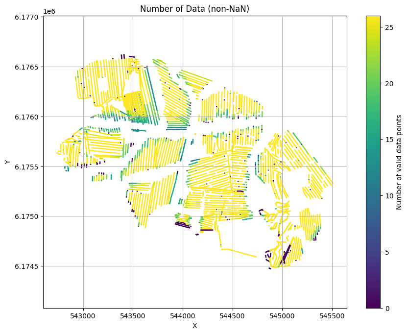
[5]:
X, Y, LINE, ELEVATION = ig.get_geometry(f_data_h5)
with h5py.File(f_data_h5, 'r') as f_data:
NON_NAN = np.sum(~np.isnan(f_data['/D1/d_obs']), axis=1)
# --- Strategy A: use the most-common survey line number ---
unique_lines, counts = np.unique(LINE, return_counts=True)
most_frequent_line = unique_lines[np.argmax(counts)]
print("Most frequent line number:", most_frequent_line)
id_line_A = np.where(LINE == most_frequent_line)[0]
# Trim to the first continuous run of consecutive indices
diff = np.diff(id_line_A)
cut = np.where(diff > 2)[0]
if len(cut) > 0:
id_line_A = id_line_A[: cut[0] + 1]
# --- Strategy B: spatial buffer along UTM coordinates ---
Xl = np.array([544500, 543150])
Yl = np.array([6175000, 6176500])
id_line_B, _, _ = ig.find_points_along_line_segments(
X, Y, Xl, Yl, tolerance=10.0
)
# Use strategy B as the default profile line for all examples below
id_line = id_line_B
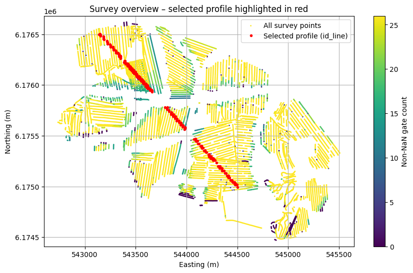
# Map showing the selected profile
plt.figure(figsize=(10, 6))
plt.scatter(X, Y, c=NON_NAN, s=1, label='All survey points')
plt.plot(X[id_line], Y[id_line], 'r.', markersize=6,
label='Selected profile (id_line)', zorder=2)
plt.colorbar(label='Non-NaN gate count')
plt.xlabel('Easting (m)')
plt.ylabel('Northing (m)')
plt.title('Survey overview – selected profile highlighted in red')
plt.axis('equal')
plt.legend()
plt.grid(True)
if hardcopy:
plt.savefig('profile_survey_overview.png', dpi=300)
plt.show()
Most frequent line number: 150.0
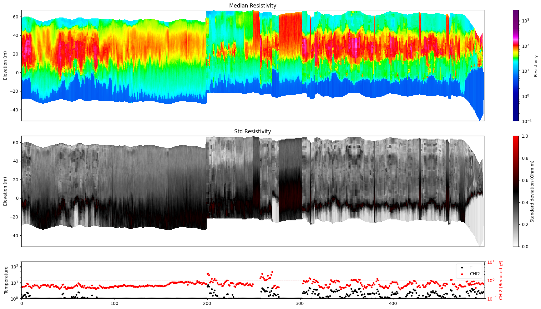
3. X-axis choices
The horizontal axis of the profile cross-section can show different coordinate types. All remaining examples use xaxis='x' (UTM easting) because it gives physically meaningful spacing.
|
Description |
|---|---|
|
Renumbered sequential indices 0, 1, 2, … (default) |
|
Original data-point IDs from the file |
|
UTM easting (metres) |
|
UTM northing (metres) |
[6]:
ig.plot_profile(f_post_h5, im=1, ii=id_line, xaxis='index')
Getting cmap from attribute
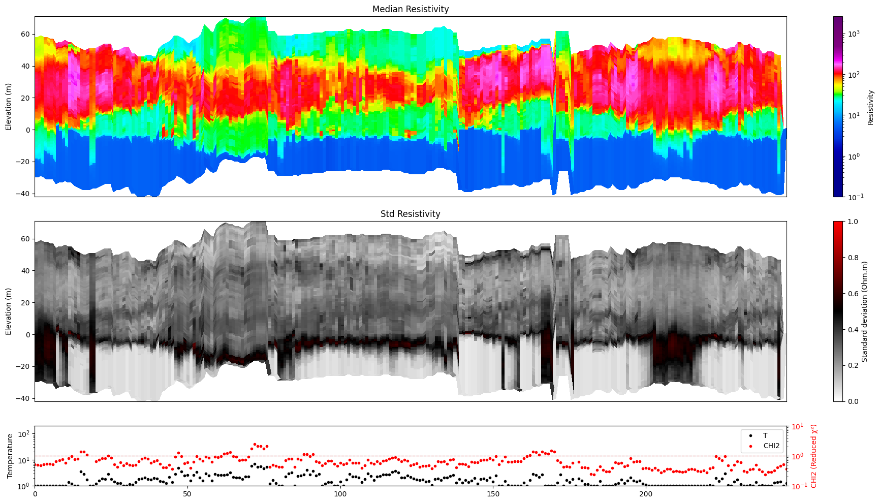
[7]:
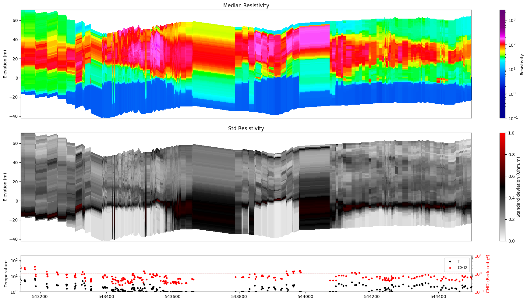
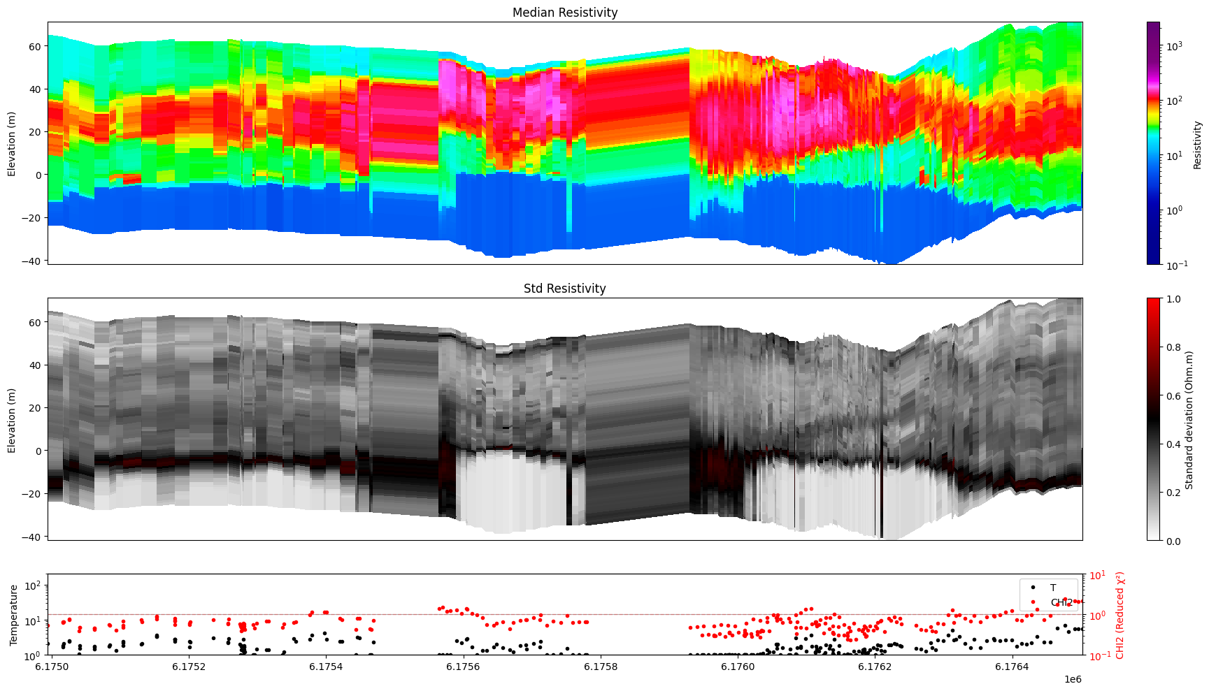
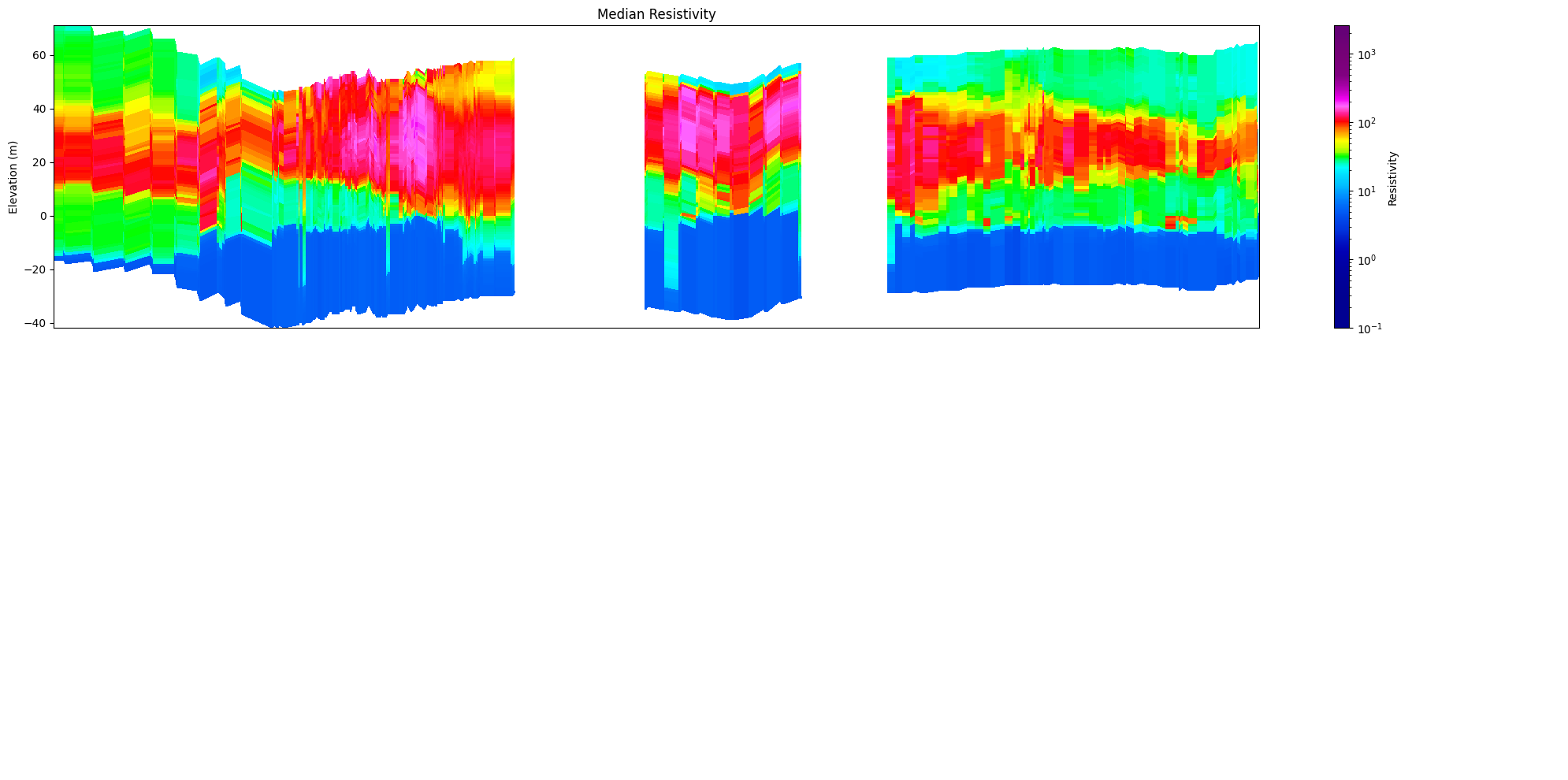
ig.plot_profile(f_post_h5, im=1, ii=id_line, xaxis='x')
Getting cmap from attribute
[8]:
ig.plot_profile(f_post_h5, im=1, ii=id_line, xaxis='y')
Getting cmap from attribute
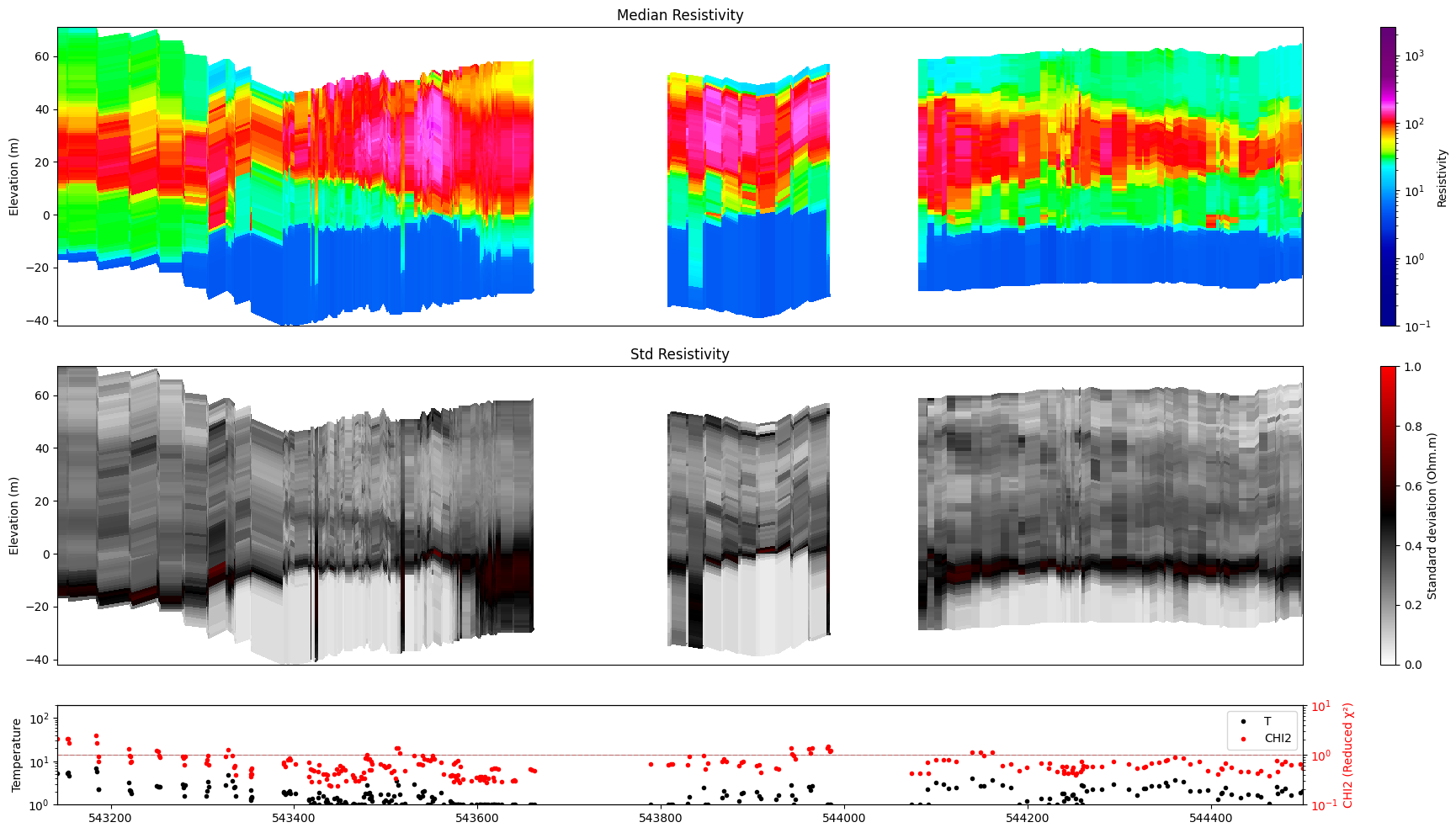
4. Handling spatial gaps
When the selected points are not all adjacent (e.g. data from multiple flight lines are concatenated) a gap_threshold renders the discontinuous regions fully transparent, making line breaks clearly visible.
The threshold is expressed in the same units as the chosen x-axis: metres for 'x' / 'y', point count for 'index'.
[9]:
ig.plot_profile(f_post_h5, im=1, ii=id_line, xaxis='x', gap_threshold=50)
Getting cmap from attribute

[10]:
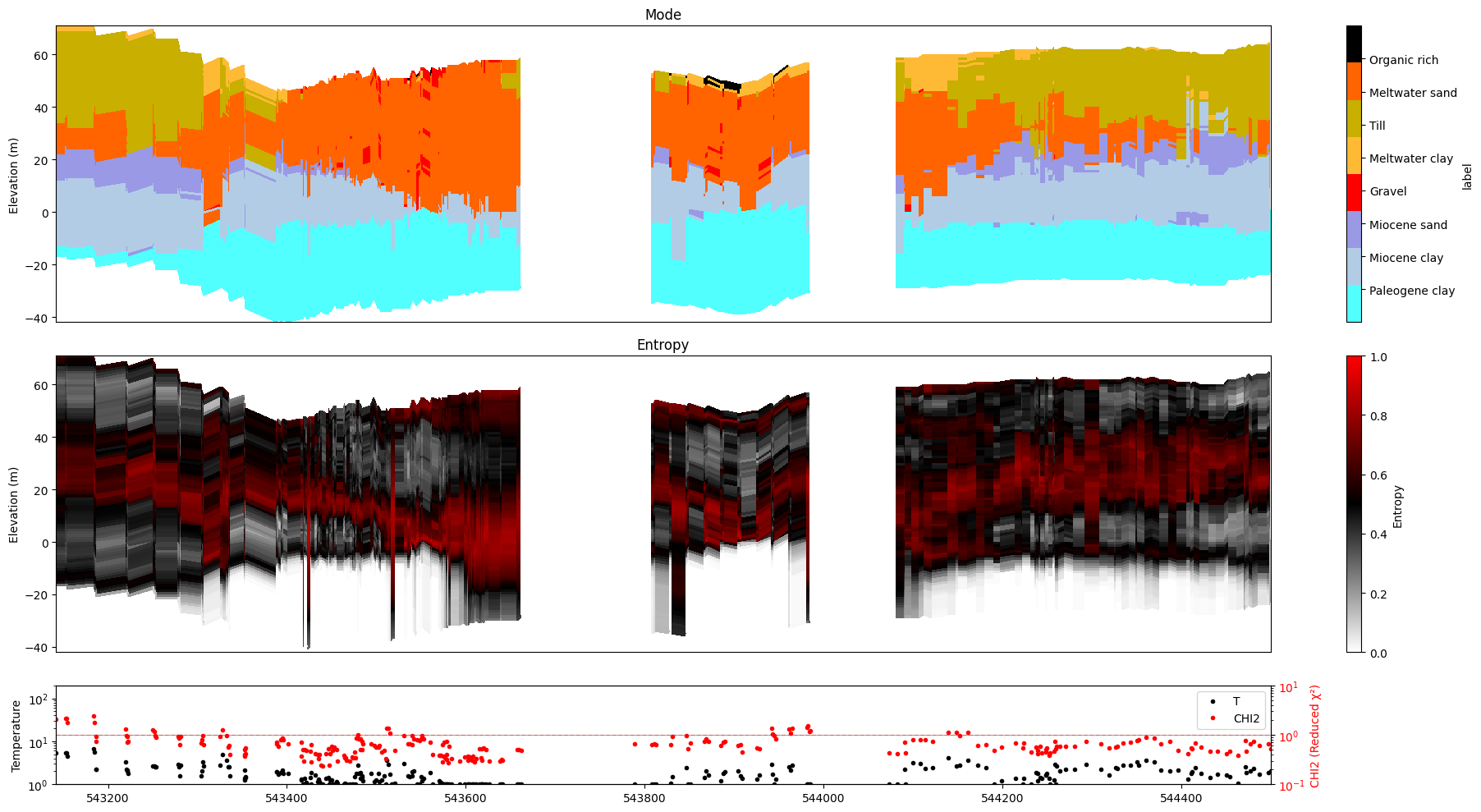
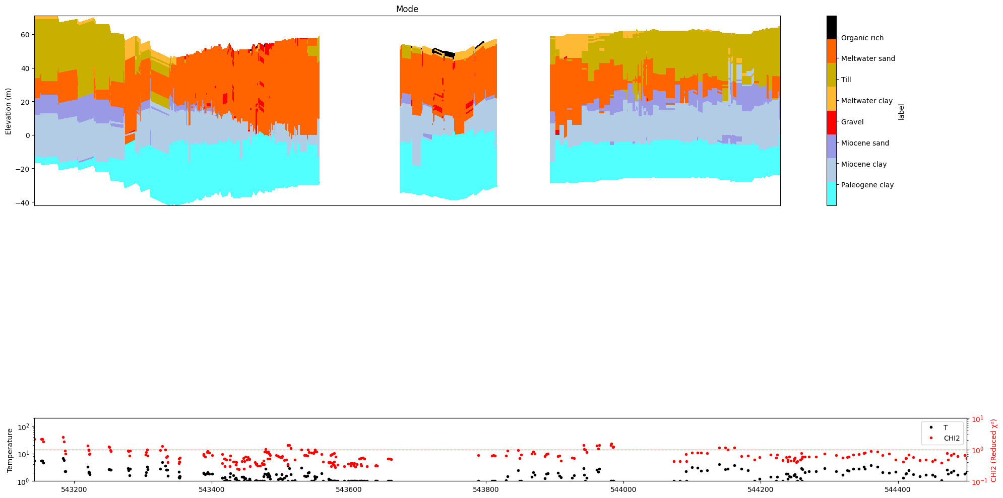
ig.plot_profile(f_post_h5, im=2, ii=id_line, xaxis='x', gap_threshold=50)
All examples from here on use ``ii=id_line`` and ``xaxis=’x’`` |
as the standard spatial profile configuration. |
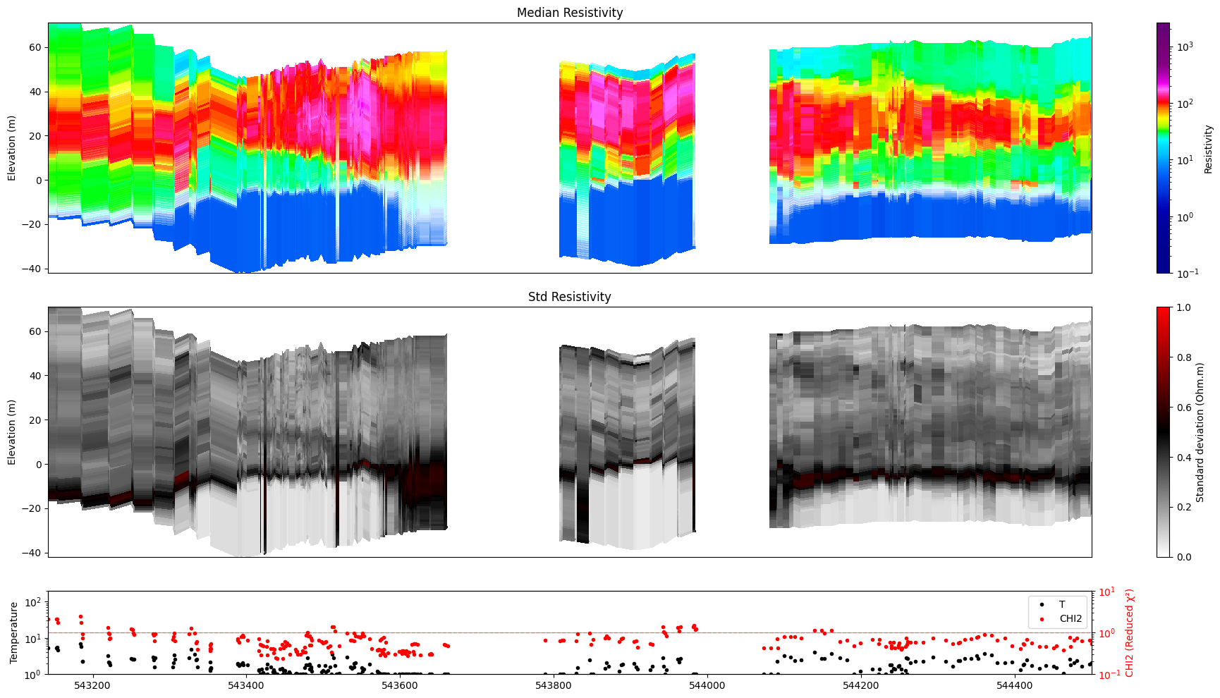
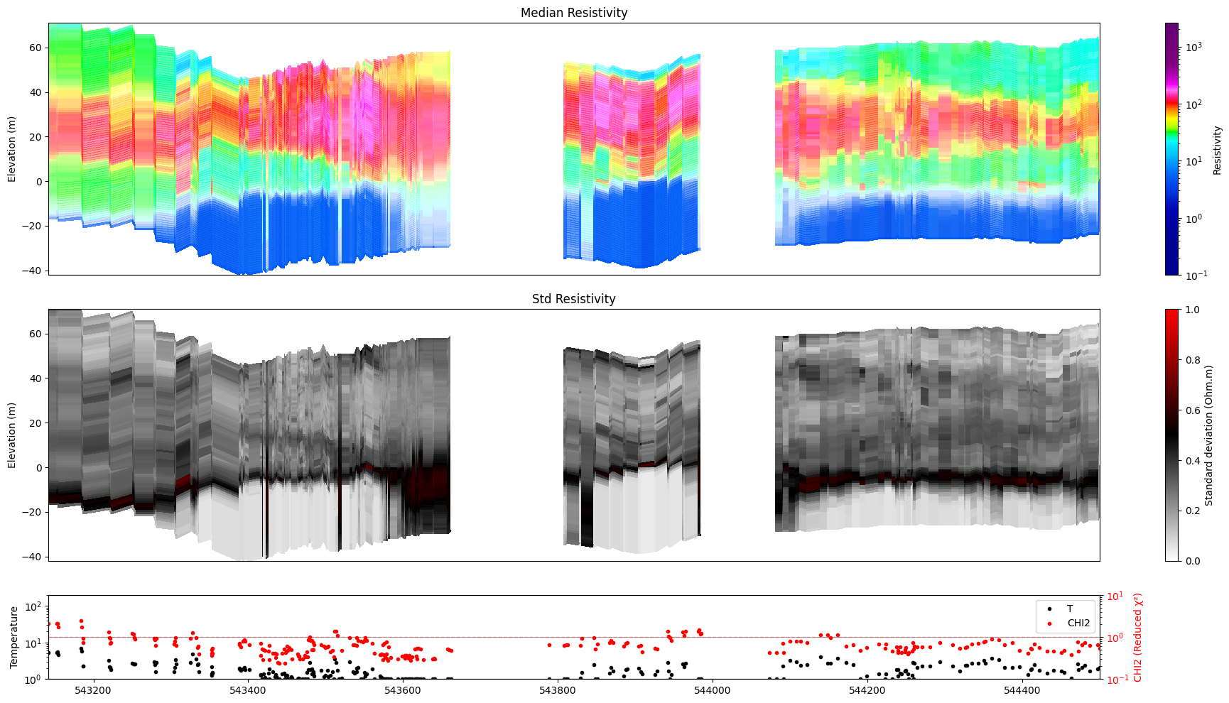
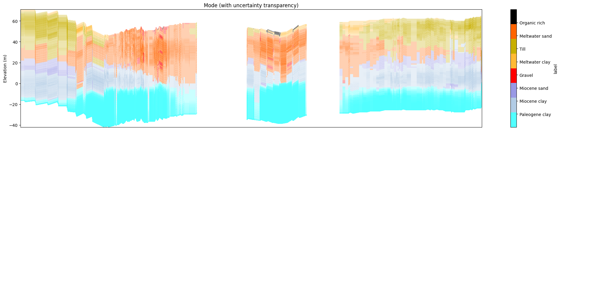
5. Selecting a single model
Use im=1, im=2, … to target a specific model in the posterior file.
M1 – continuous resistivity (log-resistivity layers)
M2 – discrete lithology classes
[11]:
ig.plot_profile(f_post_h5, im=1, ii=id_line, xaxis='x', gap_threshold=50)
Getting cmap from attribute
[12]:
ig.plot_profile(f_post_h5, im=2, ii=id_line, xaxis='x', gap_threshold=50)

6. All models at once
im=0 (the default) detects every model stored in the posterior file and produces one figure per model automatically.
[13]:
ig.plot_profile(f_post_h5, im=0, ii=id_line, xaxis='x', gap_threshold=50)
Plot profile for all model parameters
Getting cmap from attribute


Only nm=1, model parameters. no profile will be plot
7. Index-range selection as an alternative to ii=
When you just want a quick look at a contiguous block of data points you can use i1 / i2 instead of building an explicit index array.
Method |
How to use |
Notes |
|---|---|---|
|
|
1-based inclusive range |
|
|
Arbitrary array; overrides |
[14]:
ig.plot_profile(f_post_h5, im=1, i1=1, i2=500)
Getting cmap from attribute
[15]:
ig.plot_profile(f_post_h5, im=1, ii=id_line[::2], xaxis='x', gap_threshold=50)
Getting cmap from attribute

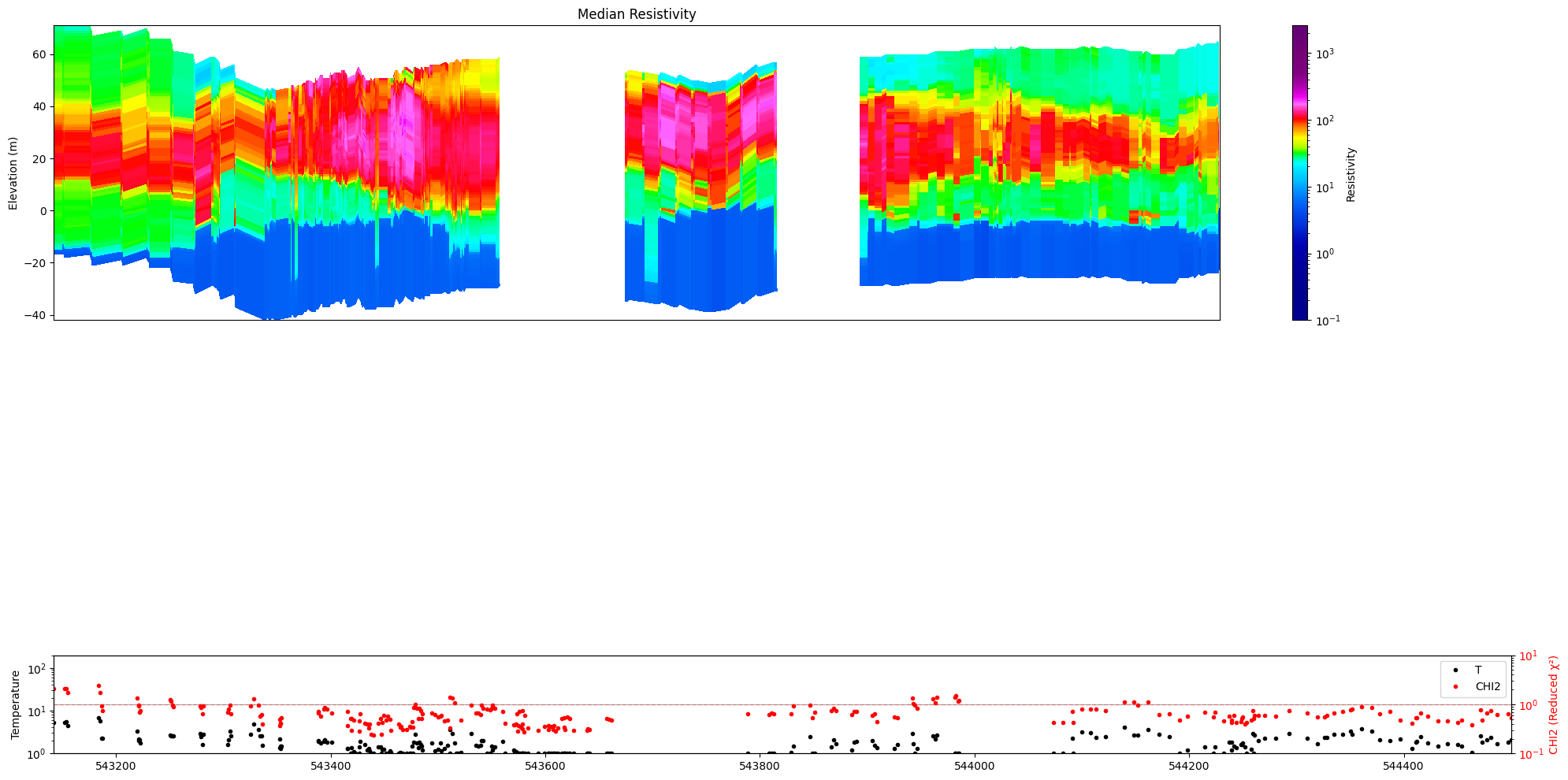
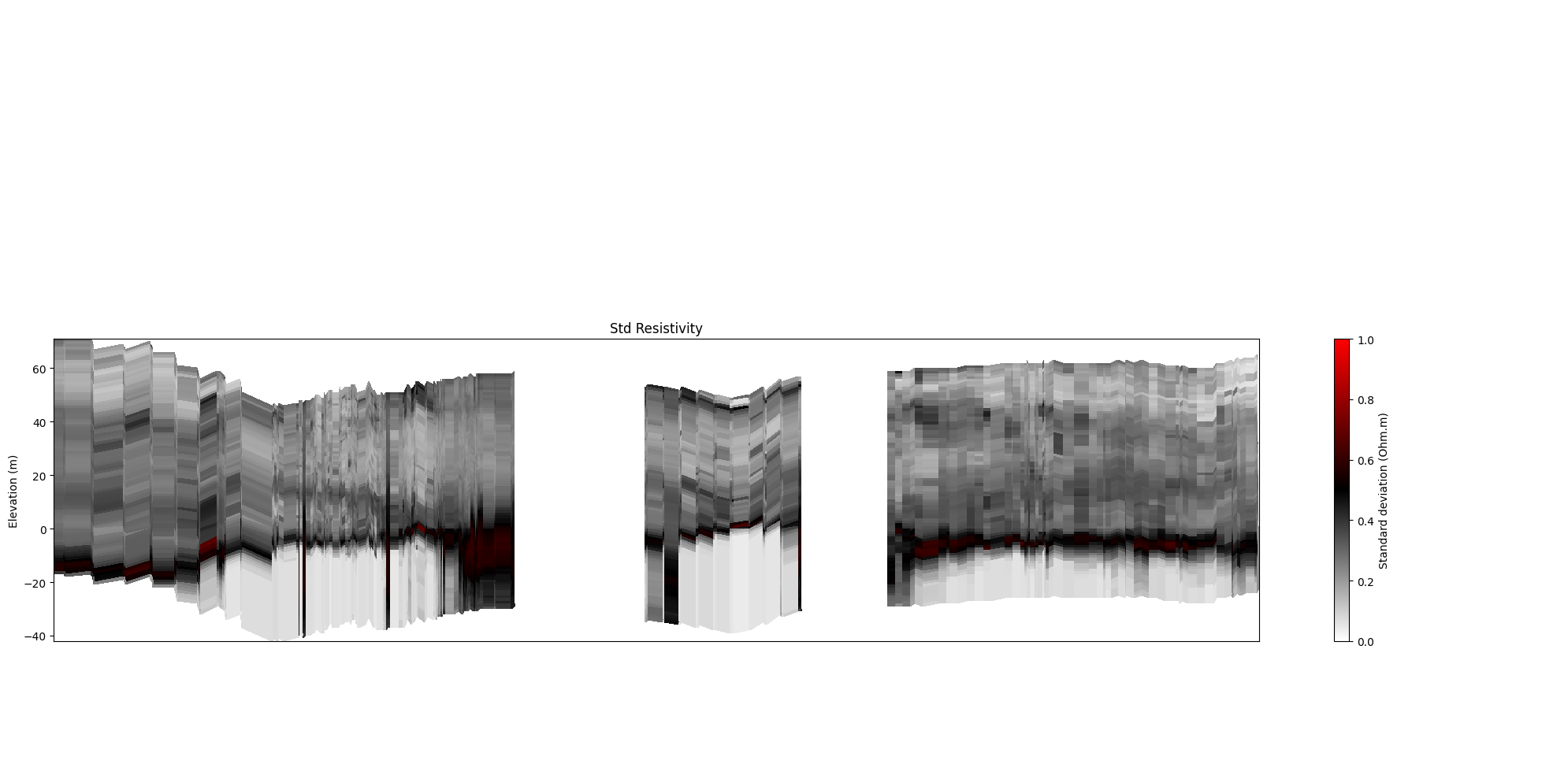
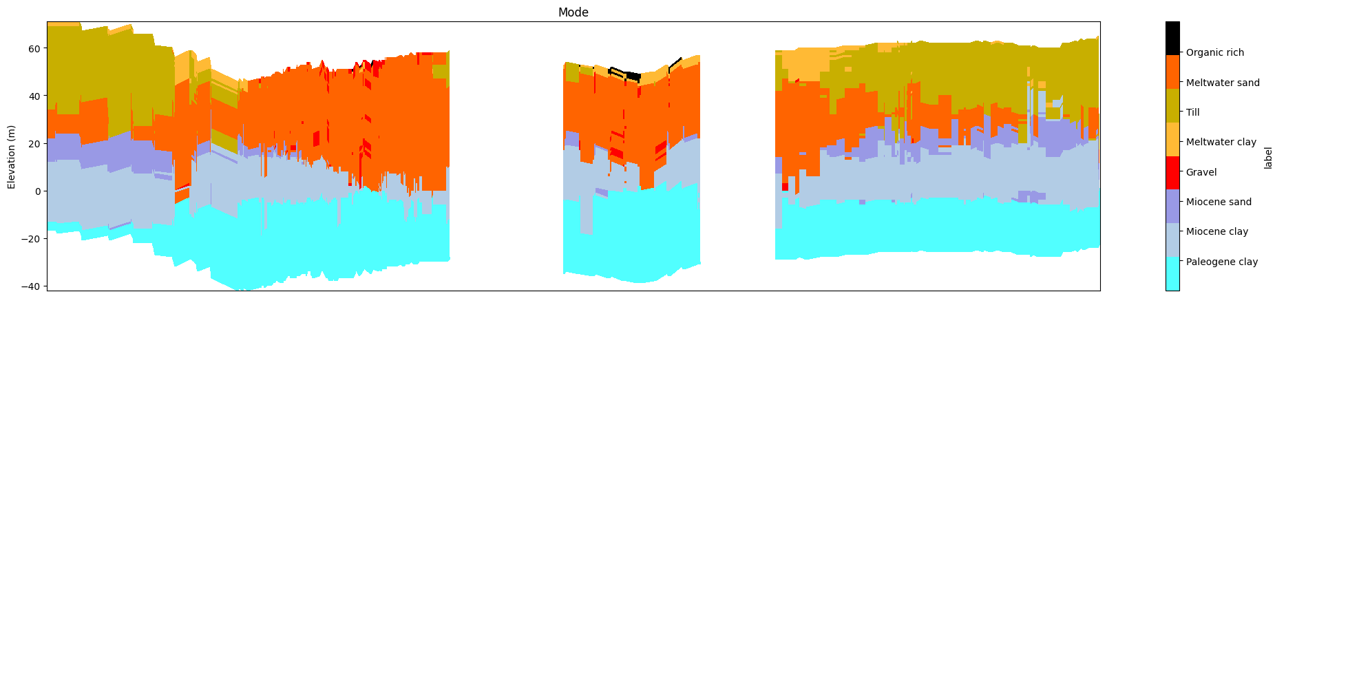
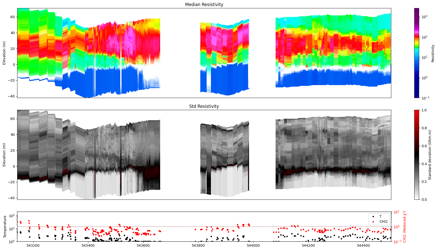
8. Choosing individual panels
Pass panels= to show only a subset of the three panels.
Continuous models – available panels: 'value', 'std', 'stats' (aliases: 'median'/'mean' → 'value'; 'uncertainty' → 'std'; 't'/'temperature' → 'stats')
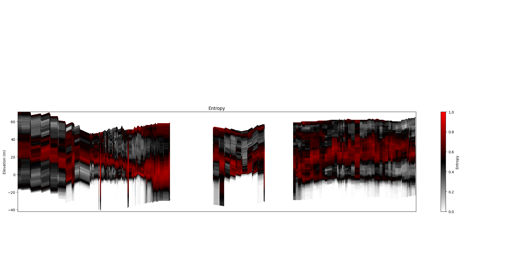
Discrete models – available panels: 'mode', 'entropy', 'stats' (alias: 't'/'temperature' → 'stats')
[16]:
ig.plot_profile(f_post_h5, im=1, ii=id_line, xaxis='x',  gap_threshold=50,
                panels=['value'])
Getting cmap from attribute
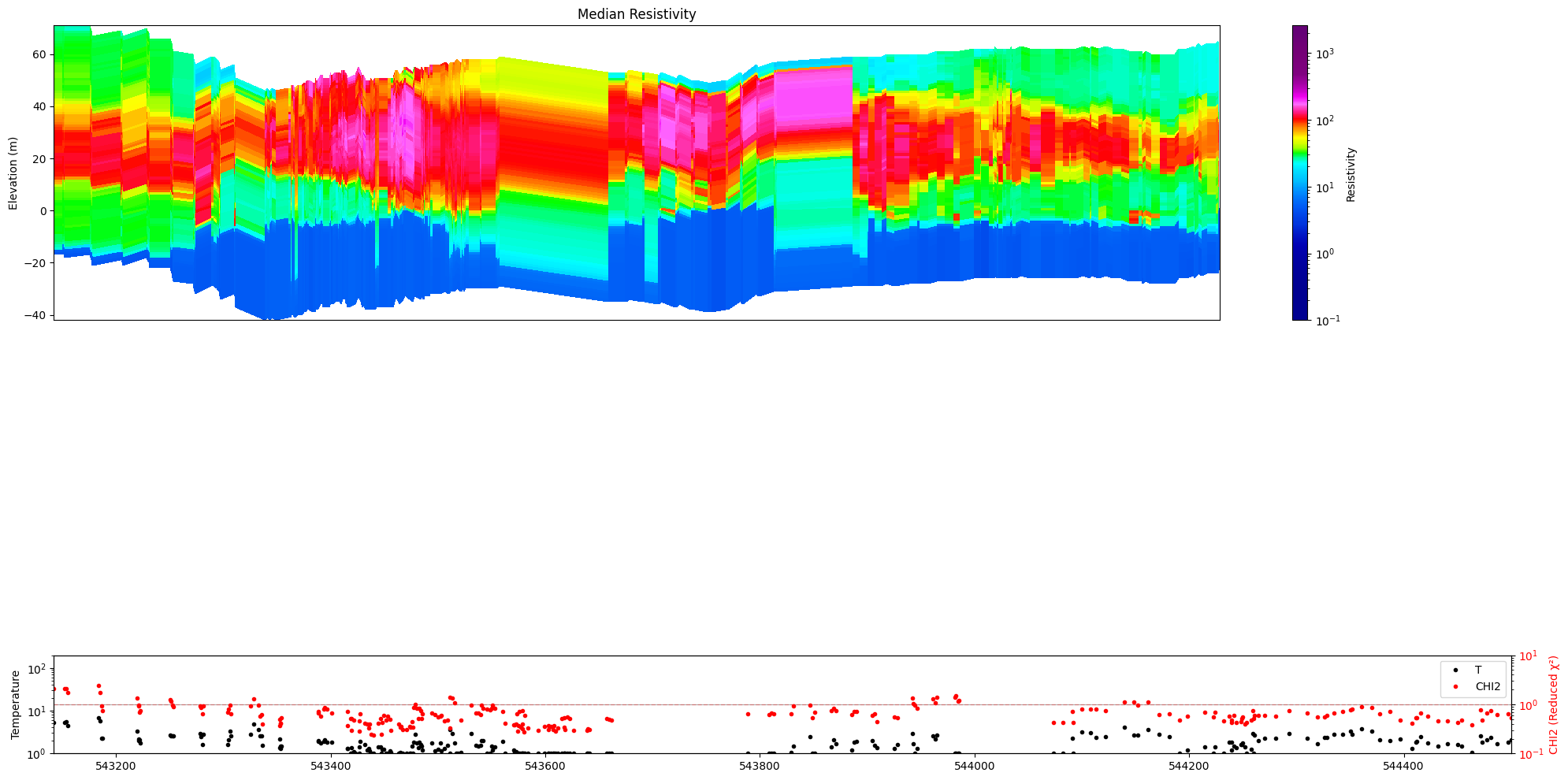
[17]:
ig.plot_profile(f_post_h5, im=1, ii=id_line, xaxis='x', gap_threshold=50,
                panels=['value', 'stats'])
Getting cmap from attribute
[18]:
ig.plot_profile(f_post_h5, im=1, ii=id_line, xaxis='x',  gap_threshold=50,
                panels=['std'])
Getting cmap from attribute
[19]:
ig.plot_profile(f_post_h5, im=2, ii=id_line, xaxis='x', gap_threshold=50,
                panels=['mode'])
[20]:
ig.plot_profile(f_post_h5, im=2, ii=id_line, xaxis='x', gap_threshold=50,
                panels=['mode', 'stats'])
[21]:
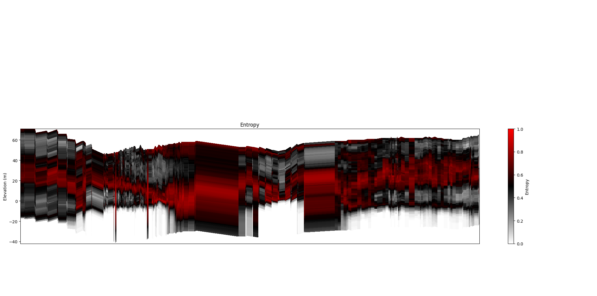
ig.plot_profile(f_post_h5, im=2, ii=id_line, xaxis='x', gap_threshold=50,
                panels=['entropy'])
9. Uncertainty transparency
alpha (0–1) fades out uncertain regions in the primary panel:
M1 (continuous): driven by standard deviation
M2 (discrete): driven by entropy
alpha=0 → fully opaque everywhere (default) alpha=1 → maximum fade where uncertainty is highest
[ ]:
[22]:
ig.plot_profile(f_post_h5, im=1, ii=id_line, xaxis='x',
                alpha=1, gap_threshold=50, std_min=0.3, std_max=0.5)
Getting cmap from attribute
0.0
1.0
[23]:
ig.plot_profile(f_post_h5, im=1, ii=id_line, xaxis='x',
                alpha=0.8, gap_threshold=50, std_min=0.3, std_max=0.5)
Getting cmap from attribute
0.19999999
1.0
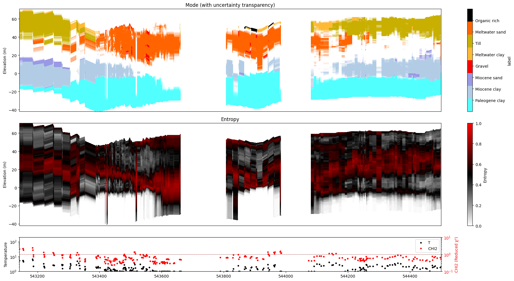
[24]:
ig.plot_profile(f_post_h5, im=2, ii=id_line, xaxis='x',
                alpha=1.0, entropy_min=0.5, entropy_max=0.6,
                gap_threshold=50)
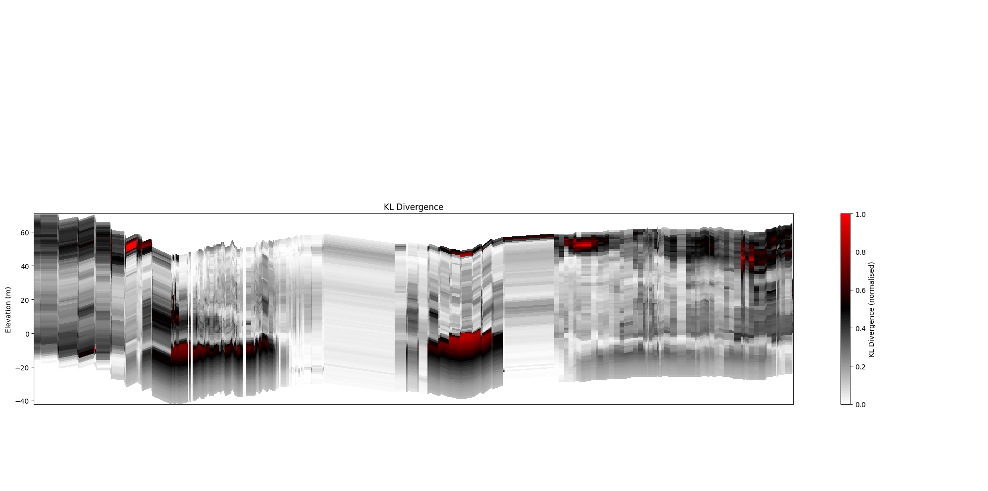
10. KL divergence
KL divergence measures how much the posterior distribution differs from the prior. It is stored under Mx/KL in the posterior file after running ig.integrate_posterior_stats(..., computeKL=True).
plot_kl=True substitutes it for the uncertainty panel:
M1: replaces Std
M2: replaces Entropy
If Mx/KL is absent the function falls back to the standard panel with a warning.
[25]:
# ig.integrate_posterior_stats(f_post_h5, computeKL=True)
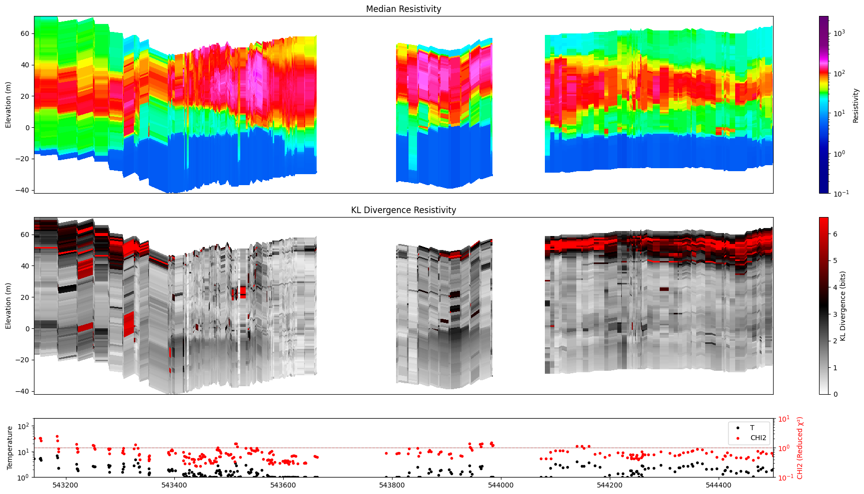
[26]:
ig.plot_profile(f_post_h5, im=1, ii=id_line, xaxis='x',
                gap_threshold=50, plot_kl=True )
#ig.integrate_posterior_stats(f_post_h5)
Getting cmap from attribute
/home/au11687/integrate/lib/python3.12/site-packages/numpy/lib/_function_base_impl.py:4786: UserWarning: Warning: 'partition' will ignore the 'mask' of the MaskedArray.
  arr.partition(
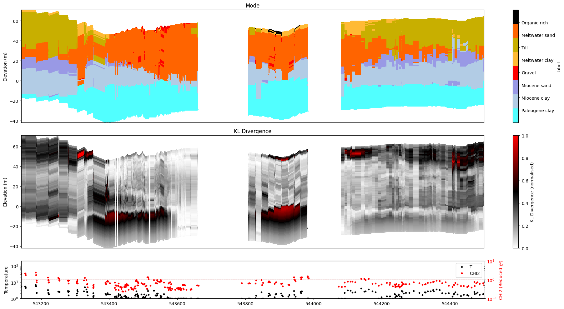
[27]:
ig.plot_profile(f_post_h5, im=2, ii=id_line, xaxis='x',
                plot_kl=True, gap_threshold=50)
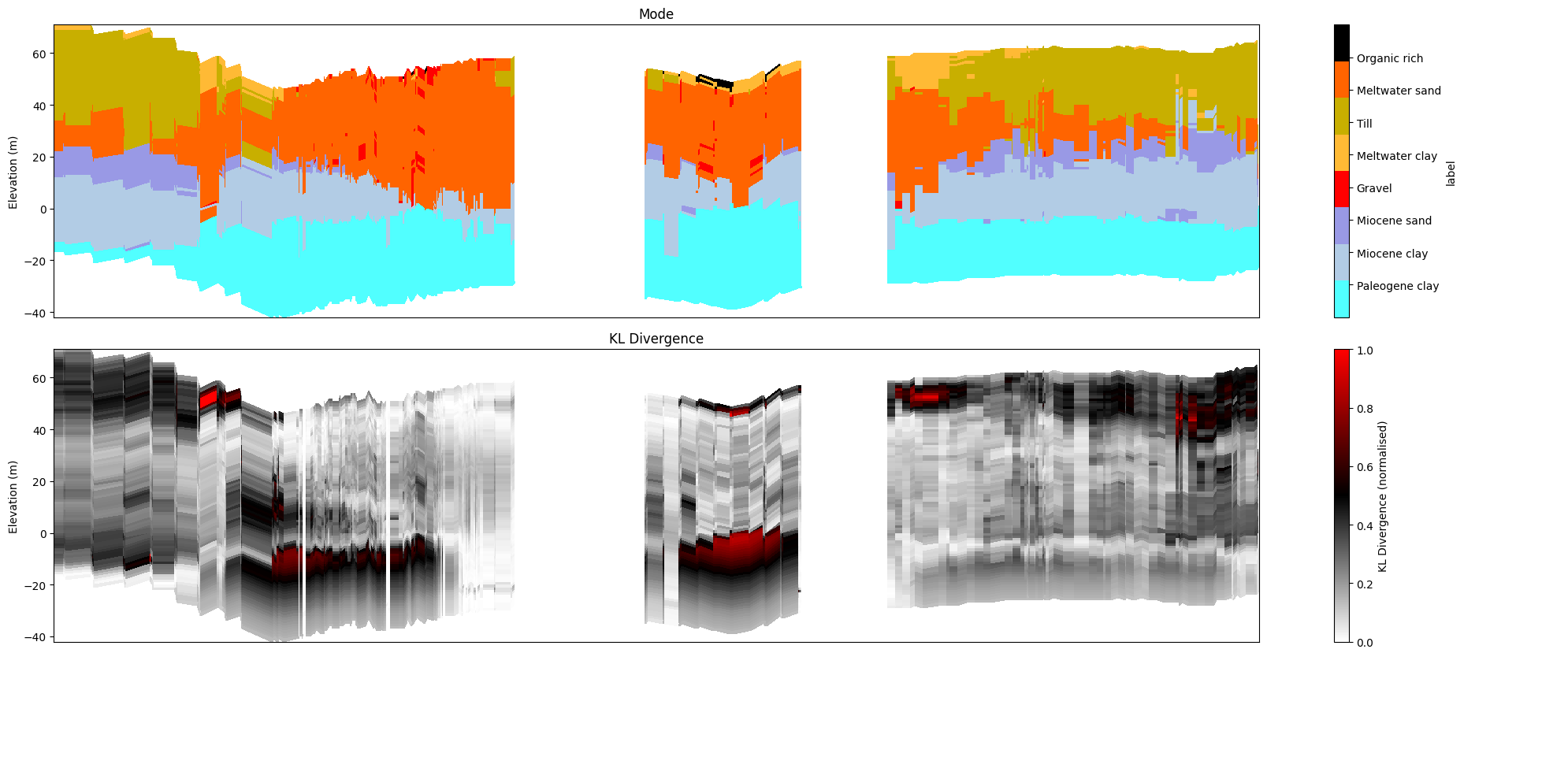
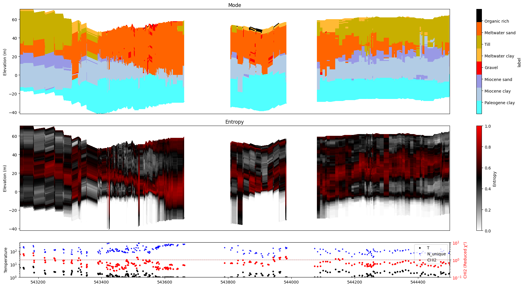
[28]:
ig.plot_profile(f_post_h5, im=2, ii=id_line, xaxis='x',
                panels=['mode', 'entropy'],
                plot_kl=True, gap_threshold=50)
[29]:
ig.plot_profile(f_post_h5, im=2, ii=id_line, xaxis='x',
                panels=['entropy'], plot_kl=False)
ig.plot_profile(f_post_h5, im=2, ii=id_line, xaxis='x',
                panels=['entropy'], plot_kl=True)
plt.show()
11. Number of unique realizations
show_n_unique=True overlays the count of distinct accepted posterior realizations at each location onto the stats panel. Requires N_UNIQUE to be stored in the posterior file.
[30]:
ig.plot_profile(f_post_h5, im=1, ii=id_line, xaxis='x',
                show_n_unique=True, gap_threshold=50)
Getting cmap from attribute

[31]:
ig.plot_profile(f_post_h5, im=2, ii=id_line, xaxis='x',
                show_n_unique=True, gap_threshold=50)
12. Saving figures to disk
hardcopy=True writes a PNG file with an auto-generated name derived from the posterior file name, model index, and index range. Use txt= to append a custom suffix.
[32]:
ig.plot_profile(f_post_h5, im=1, ii=id_line, xaxis='x',
                gap_threshold=50,
                hardcopy=True)
Getting cmap from attribute

[33]:
ig.plot_profile(f_post_h5, im=1, ii=id_line, xaxis='x',
                panels=['value', 'stats'],
                hardcopy=True, txt='value_only')
Getting cmap from attribute
[34]:
ig.plot_profile(f_post_h5, im=2, ii=id_line, xaxis='x',
                plot_kl=True, gap_threshold=50,
                hardcopy=True, txt='kl')

13. Combined options
Putting it all together for publication-quality figures.
[35]:
ig.plot_profile(f_post_h5, im=1, ii=id_line, xaxis='x',
                alpha=0.8, gap_threshold=50,
                hardcopy=hardcopy)
Getting cmap from attribute
0.19999999
1.0
[36]:
ig.plot_profile(f_post_h5, im=2, ii=id_line, xaxis='x',
                plot_kl=True, gap_threshold=50,
                hardcopy=hardcopy)

[37]:
ig.plot_profile(f_post_h5, im=1, ii=id_line, xaxis='x',
                panels=['value', 'stats'],
                show_n_unique=True, gap_threshold=50)
Getting cmap from attribute

[38]:
ig.plot_profile(f_post_h5, im=2, ii=id_line, xaxis='x',
                panels=['mode'],
                alpha=0.7, gap_threshold=50)
[39]:
ig.plot_profile(f_post_h5, im=0, ii=id_line, xaxis='x',
                plot_kl=True, gap_threshold=50,
                hardcopy=hardcopy)
Plot profile for all model parameters
Getting cmap from attribute
/home/au11687/integrate/lib/python3.12/site-packages/numpy/lib/_function_base_impl.py:4786: UserWarning: Warning: 'partition' will ignore the 'mask' of the MaskedArray.
  arr.partition(


Only nm=1, model parameters. no profile will be plot
Summary of key plot_profile() options
Option |
Values |
Effect |
|---|---|---|
|
|
Select model; 0 plots all |
|
array |
Explicit index selection (overrides |
|
int |
1-based range, alternative to |
|
|
Horizontal axis type |
|
float |
Mark gaps beyond this distance as transparent |
|
0–1 |
Uncertainty-driven transparency of primary panel |
|
list of str |
Subset of panels to show |
|
bool |
KL divergence instead of entropy / std |
|
bool |
Overlay N_unique on stats panel |
|
bool |
Save PNG file |
|
str |
Suffix appended to auto-generated filename |