query: Posterior Query Tool

Computes the probability, per data point, that posterior realizations satisfy a user-defined feature constraint.

The core function query(f_post_h5, query) takes a posterior HDF5 file and a query definition (dict or JSON file path) and returns an array of

probabilities – one value per data location.

try:
    get_ipython()
    get_ipython().run_line_magic('load_ext', 'autoreload')
    get_ipython().run_line_magic('autoreload', '2')
except Exception:
    pass

import json

import h5py
import numpy as np
import matplotlib.pyplot as plt
import integrate as ig

Query structure

A query is a dict (or JSON file) with a "constraints" list. Constraints are evaluated sequentially (implicit AND): a realization must pass all constraints to be counted.

Discrete-model constraint (e.g. lithology class, im=2)

{
  "im": 2,
  "classes": [1, 2],
  "thickness_mode": "cumulative",
  "thickness_comparison": ">",
  "thickness_threshold": 10.0,
  "depth_min": 0.0,
  "depth_max": 30.0,
  "negate": false
}

Continuous-model constraint (e.g. resistivity, im=1)

{
  "im": 1,
  "value_comparison": "<",
  "value_threshold": 500.0,
  "thickness_mode": "cumulative",
  "thickness_comparison": ">",
  "thickness_threshold": 0.0,
  "depth_min": 0.0,
  "depth_max": 100.0,
  "negate": false
}

All fields:

Field	Type	Description
im	int	Prior model index (1-based)
classes	list[int]	Class IDs to match (discrete only)
value_comparison	str	"<" or ">" (continuous only)
value_threshold	float	Value threshold for continuous condition
thickness_mode	str	"cumulative" or "first_occurrence"
thickness_comparison	str	">", "<", ">=", "<="
thickness_threshold	float	Thickness [m] to compare against
depth_min	float	Optional lower depth bound [m]
depth_max	float	Optional upper depth bound [m]
negate	bool	If True, accept realizations that do NOT satisfy the constraint

---

Core Functions

The core query functions (query, query_plot, save_query, load_query, get_prior_model_info) are available from the integrate module. Access them as:

• ig.query()

• ig.query_plot()

• ig.save_query()

• ig.load_query()

• ig.get_prior_model_info()

All helper functions and implementation details are in integrate/integrate_query.py

---

Examples

The examples below use the posterior and prior files from the examples/ directory. They are guarded with os.path.isfile so the script can be imported without errors if the files are absent. import integrate as ig f_post_h5 = ‘post_daugaard_merged_N2000000_Nuse1000000_inflateNoise2.h5’ with h5py.File(f_post_h5, ‘r’) as f: f_prior_h5 = str(f.attrs.get(‘f5_prior’, ‘’)) f_data_h5 = str(f.attrs.get(‘f5_data’, ‘’)) X, Y, LINE, ELEVATION = ig.get_geometry(f_data_h5)

z = [] dz = [] with h5py.File(f_prior_h5, ‘r’) as f: for k in f.keys(): if k.startswith(‘M’): z.append(f[k].attrs[‘x’].astype(float)) # dz = [diff(z),0] dz.append(np.append(np.diff(z[-1]), 0))

ig.plot_profile(f_post_h5, i1 = 0, i2=600, im=2) M, idx = ig.load_prior_model(f_prior_h5)

# Select posterior hdf5 file to query
# (here an example the outcome og integrate_workflow.py)
f_post_h5= 'post_DAUGAARD_AVG_WF_id1_2_3_4_5_6_7_8_9_10_11_12_13.h5'
# Select data location to plot
ip = 1000

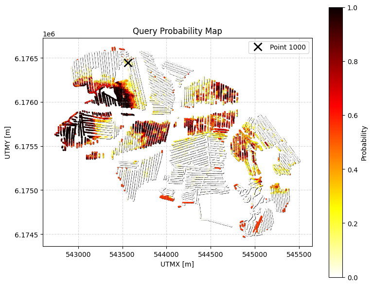
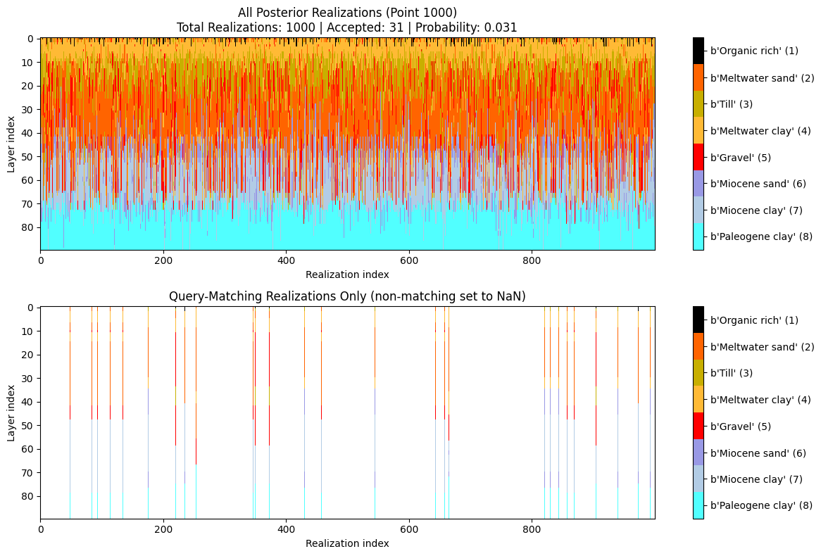
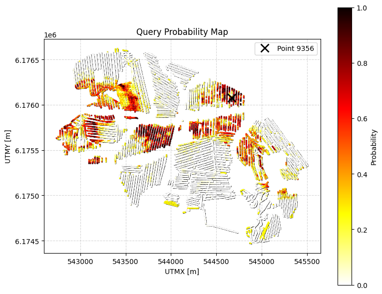
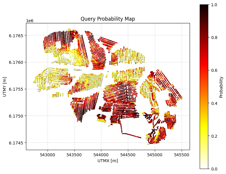
Example 1: Discrete constraint

Probability that the cumulative thickness of lithology class 2 within 0–30 m depth is greater than 10 m.

# Q0: FIND THE TOTAL AMOUNT OF SAND and GRAVEL above 30 m depth!
query_ex0 = {
    "constraints": [
        {
            "im": 2,
            "classes": [2,5],
            "thickness_mode": "cumulative",
            "thickness_comparison": ">",
            "thickness_threshold": 20.0,
            "depth_min": 0.0,
            "depth_max": 30.0,
            "negate": False
        }
    ]
}

ig.save_query(query_ex0, 'query_ex0.json')

P0, meta0 = ig.query(f_post_h5, query_ex0)
print(f"Example 0 | N_data={meta0['N_data']}, mean P={P0.mean():.3f}")

# Simple: just probability map
# ig.query_plot(P0, meta0)

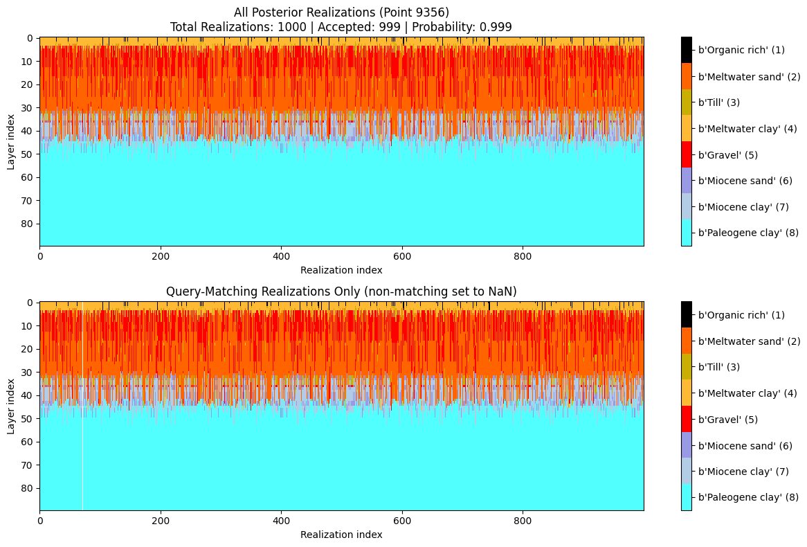
# Detailed: probability map + model visualization for point 1000
ig.query_plot(P0, meta0, ip=ip, query_dict=query_ex0, f_post_h5=f_post_h5)

Query saved to query_ex0.json

Evaluating query: 100%|██████████████████████████████████████████████████████████████████████| 11693/11693 [00:01<00:00, 6649.48location/s]

Example 0 | N_data=11693, mean P=0.277

# Pause execution here to allow inspection of the plots before the script continues
#input("Press Enter to continue with manual computation...")

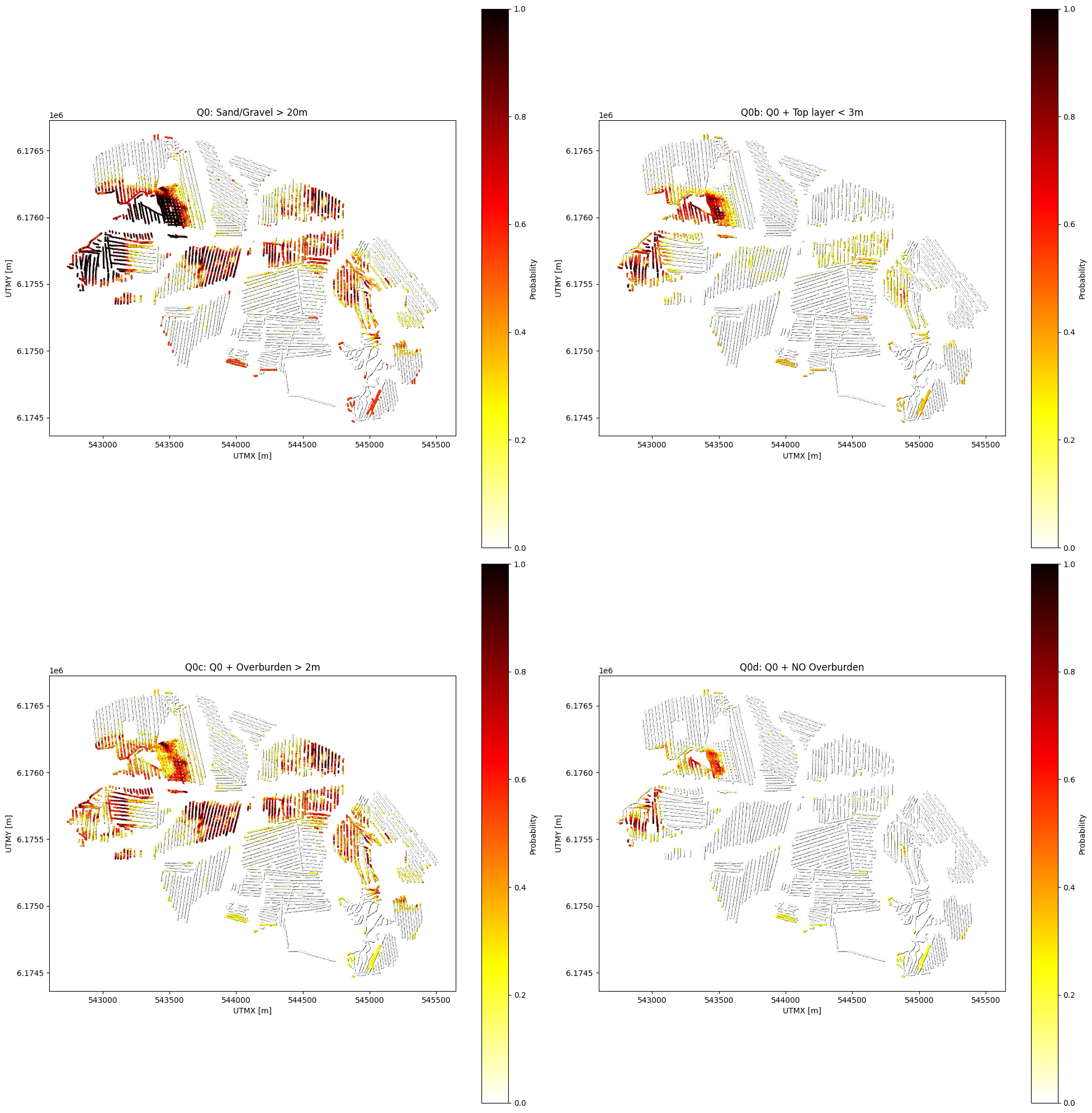
Example 0b: Q0 with additional constraint on top layer thickness

Same as Q0 (sand and gravel cumulative thickness > 20m within 0-30m) BUT with an additional constraint: any top layer that is NOT sand/gravel cannot be thicker than 3m.

query_ex0b = {
    "constraints": [
        {
            "im": 2,
            "classes": [2, 5],
            "thickness_mode": "cumulative",
            "thickness_comparison": ">",
            "thickness_threshold": 20.0,
            "depth_min": 0.0,
            "depth_max": 30.0,
            "negate": False
        },
        {
            "im": 2,
            "classes": [1, 3, 4, 6, 7, 8],  # All classes except sand (2) and gravel (5)
            "thickness_mode": "first_occurrence",
            "thickness_comparison": "<",
            "thickness_threshold": 3.0,
            "depth_min": 0.0,
            "depth_max": 30.0,
            "negate": False
        }
    ]
}

ig.save_query(query_ex0b, 'query_ex0b.json')

P0b, meta0b = ig.query(f_post_h5, query_ex0b)
print(f"Example 0b | N_data={meta0b['N_data']}, mean P={P0b.mean():.3f}")

# Detailed visualization for a specific point
ig.query_plot(P0b, meta0b, ip=ip, query_dict=query_ex0b, f_post_h5=f_post_h5)

Query saved to query_ex0b.json

Evaluating query: 100%|███████████████████████████████████████████████████████████████████████| 11693/11693 [00:46<00:00, 252.84location/s]

Example 0b | N_data=11693, mean P=0.101

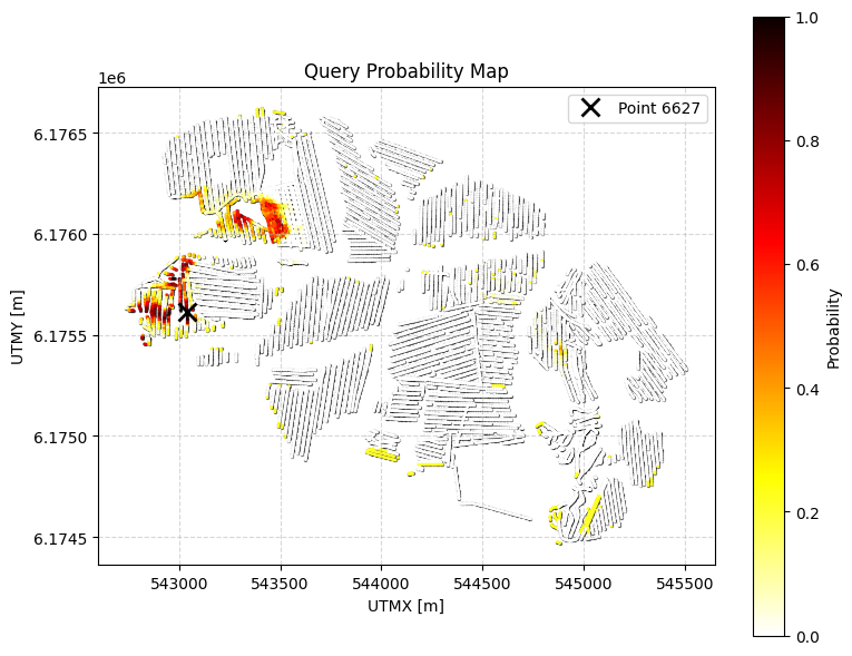
Example 0c: Q0 with minimum overburden thickness constraint

Same as Q0 (sand and gravel cumulative thickness > 20m within 0-30m) BUT with an additional constraint: there must be AT LEAST 2m of overburden (non-sand/gravel material) within 0-30m depth.

Overburden = all classes except sand (2) and gravel (5)

query_ex0c = {
    "constraints": [
        {
            "im": 2,
            "classes": [2, 5],
            "thickness_mode": "cumulative",
            "thickness_comparison": ">",
            "thickness_threshold": 20.0,
            "depth_min": 0.0,
            "depth_max": 30.0,
            "negate": False
        },
        {
            "im": 2,
            "classes": [1, 3, 4, 6, 7, 8],  # Overburden: all classes except sand (2) and gravel (5)
            "thickness_mode": "cumulative",
            "thickness_comparison": ">",
            "thickness_threshold": 2.0,
            "depth_min": 0.0,
            "depth_max": 30.0,
            "negate": False
        }
    ]
}

ig.save_query(query_ex0c, 'query_ex0c.json')

P0c, meta0c = ig.query(f_post_h5, query_ex0c)
print(f"Example 0c | N_data={meta0c['N_data']}, mean P={P0c.mean():.3f}")

#
# choose ip_example is the index of the point with laregs P0c
ip_example = np.argmax(P0c)

# Detailed visualization for a specific point
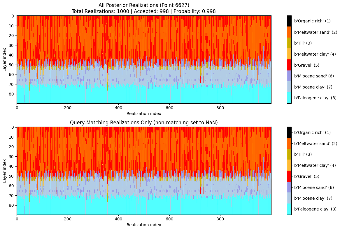
ig.query_plot(P0c, meta0c, ip=ip_example, query_dict=query_ex0c, f_post_h5=f_post_h5)

Query saved to query_ex0c.json

Evaluating query: 100%|██████████████████████████████████████████████████████████████████████| 11693/11693 [00:03<00:00, 3589.94location/s]

Example 0c | N_data=11693, mean P=0.202

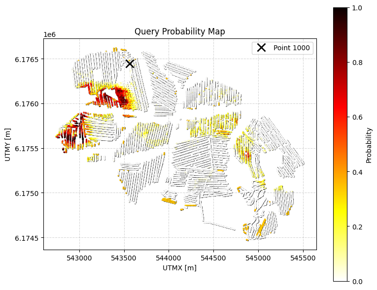
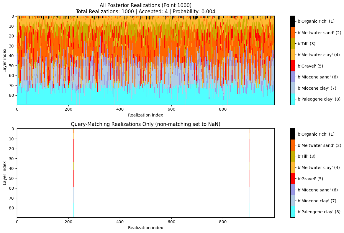
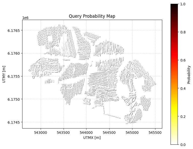
Example 0d: Q0 with NO overburden constraint

Same as Q0 (sand and gravel cumulative thickness > 20m within 0-30m) BUT with an additional constraint: there can be NO overburden at the top. This means either sand (class 2) or gravel (class 5) must be the top layer.

Overburden = all classes except sand (2) and gravel (5)

query_ex0d = {
    "constraints": [
        {
            "im": 2,
            "classes": [2, 5],
            "thickness_mode": "cumulative",
            "thickness_comparison": ">",
            "thickness_threshold": 20.0,
            "depth_min": 0.0,
            "depth_max": 30.0,
            "negate": False
        },
        {
            "im": 2,
            "classes": [1, 3, 4, 6, 7, 8],  # Overburden: all classes except sand (2) and gravel (5)
            "thickness_mode": "first_occurrence",
            "thickness_comparison": "<",
            "thickness_threshold": 0.1,  # Essentially 0 (with small numerical tolerance)
            "depth_min": 0.0,
            "depth_max": 30.0,
            "negate": False
        }
    ]
}

ig.save_query(query_ex0d, 'query_ex0d.json')

P0d, meta0d = ig.query(f_post_h5, query_ex0d)
print(f"Example 0d | N_data={meta0d['N_data']}, mean P={P0d.mean():.3f}")

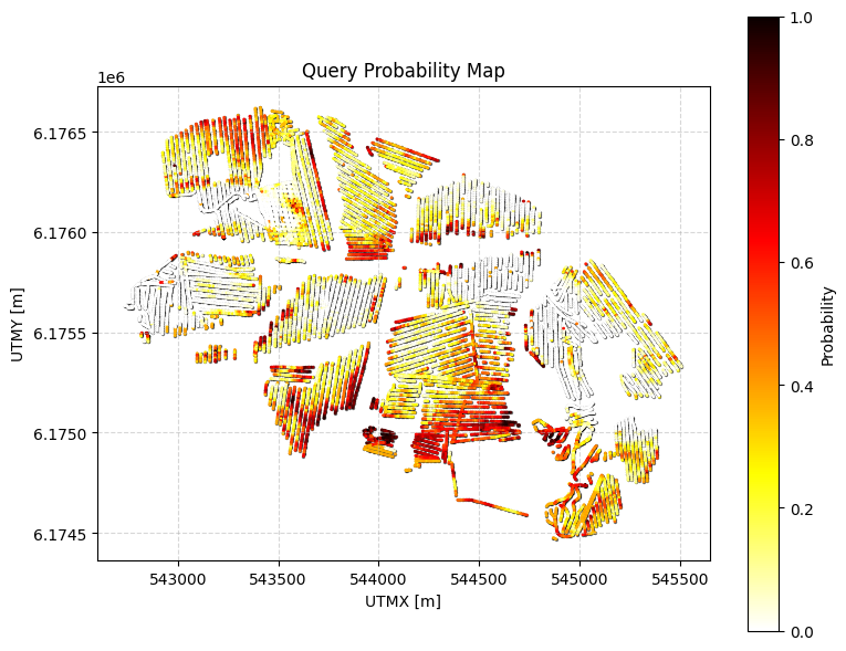
# Plot comparison: Q0, Q0b, Q0c, and Q0d
plt.figure(figsize=(20, 20))

plt.subplot(2, 2, 1)
ax1 = plt.gca()
ax1.scatter(meta0['X'], meta0['Y'], c='black', s=2, alpha=0.5)
sc1 = ax1.scatter(meta0['X'], meta0['Y'], c=P0, cmap='hot_r', vmin=0, vmax=1, s=1)
plt.colorbar(sc1, label='Probability')
plt.xlabel('UTMX [m]')
plt.ylabel('UTMY [m]')
plt.title('Q0: Sand/Gravel > 20m')
plt.gca().set_aspect('equal')

plt.subplot(2, 2, 2)
ax2 = plt.gca()
ax2.scatter(meta0b['X'], meta0b['Y'], c='black', s=2, alpha=0.5)
sc2 = ax2.scatter(meta0b['X'], meta0b['Y'], c=P0b, cmap='hot_r', vmin=0, vmax=1, s=1)
plt.colorbar(sc2, label='Probability')
plt.xlabel('UTMX [m]')
plt.ylabel('UTMY [m]')
plt.title('Q0b: Q0 + Top layer < 3m')
plt.gca().set_aspect('equal')

plt.subplot(2, 2, 3)
ax3 = plt.gca()
ax3.scatter(meta0c['X'], meta0c['Y'], c='black', s=2, alpha=0.5)
sc3 = ax3.scatter(meta0c['X'], meta0c['Y'], c=P0c, cmap='hot_r', vmin=0, vmax=1, s=1)
plt.colorbar(sc3, label='Probability')
plt.xlabel('UTMX [m]')
plt.ylabel('UTMY [m]')
plt.title('Q0c: Q0 + Overburden > 2m')
plt.gca().set_aspect('equal')

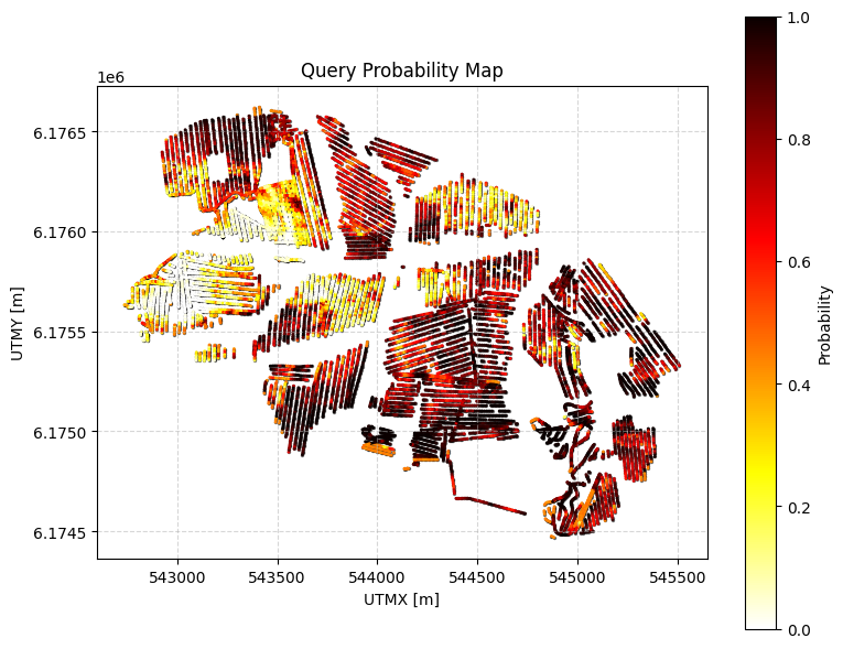
plt.subplot(2, 2, 4)
ax4 = plt.gca()
ax4.scatter(meta0d['X'], meta0d['Y'], c='black', s=2, alpha=0.5)
sc4 = ax4.scatter(meta0d['X'], meta0d['Y'], c=P0d, cmap='hot_r', vmin=0, vmax=1, s=1)
plt.colorbar(sc4, label='Probability')
plt.xlabel('UTMX [m]')
plt.ylabel('UTMY [m]')
plt.title('Q0d: Q0 + NO Overburden')
plt.gca().set_aspect('equal')

plt.tight_layout()
plt.savefig('query_example0d_comparison.png', dpi=150)
plt.show()

# Choose ip_example as the index of the point with largest P0d
ip_example = np.argmax(P0d)

# Detailed visualization for a specific point
ig.query_plot(P0d, meta0d, ip=ip_example, query_dict=query_ex0d, f_post_h5=f_post_h5)

Query saved to query_ex0d.json

Evaluating query: 100%|███████████████████████████████████████████████████████████████████████| 11693/11693 [00:46<00:00, 253.30location/s]

Example 0d | N_data=11693, mean P=0.043

query_ex1 = {
    "constraints": [
        {
            "im": 2,
            "classes": [7],
            "thickness_mode": "cumulative",
            "thickness_comparison": ">",
            "thickness_threshold": 23.0,
            "depth_min": 0.0,
            "depth_max": 100.0,
            "negate": False
        }
    ]
}

ig.save_query(query_ex1, 'query_ex1.json')

P1, meta1 = ig.query(f_post_h5, query_ex1)
print(f"Example 1 | N_data={meta1['N_data']}, mean P={P1.mean():.3f}")

ig.query_plot(P1, meta1)

Query saved to query_ex1.json

Evaluating query: 100%|██████████████████████████████████████████████████████████████████████| 11693/11693 [00:03<00:00, 3534.67location/s]

Example 1 | N_data=11693, mean P=0.248

Example 2: Continuous constraint

Probability that resistivity (im=1) is less than 100 ohm-m for a cumulative thickness of at least 5 m within 0–50 m depth.

query_ex2 = {
    "constraints": [
        {
            "im": 1,
            "value_comparison": "<",
            "value_threshold": 100.0,
            "thickness_mode": "cumulative",
            "thickness_comparison": ">",
            "thickness_threshold": 25.0,
            "depth_min": 0.0,
            "depth_max": 50.0,
            "negate": False
        }
    ]
}

ig.save_query(query_ex2, 'query_ex2.json')

P2, meta2 = ig.query(f_post_h5, query_ex2)
print(f"Example 2 | N_data={meta2['N_data']}, mean P={P2.mean():.3f}")

ig.query_plot(P2, meta2)

Query saved to query_ex2.json

Evaluating query: 100%|█████████████████████████████████████████████████████████████████████| 11693/11693 [00:00<00:00, 11946.59location/s]

Example 2 | N_data=11693, mean P=0.641

Example 3: Combined constraint (AND)

Probability that:

1. Clay (class 2) cumulative thickness > 5 m within 0–20 m, AND

2. Resistivity > 500 ohm-m for at least 1 m within 20–60 m (negated: no such layer → probability of the opposite).

query_ex3 = {
    "constraints": [
        {
            "im": 2,
            "classes": [2],
            "thickness_mode": "cumulative",
            "thickness_comparison": ">",
            "thickness_threshold": 5.0,
            "depth_min": 0.0,
            "depth_max": 20.0,
            "negate": False
        },
        {
            "im": 1,
            "value_comparison": ">",
            "value_threshold": 500.0,
            "thickness_mode": "cumulative",
            "thickness_comparison": ">",
            "thickness_threshold": 1.0,
            "depth_min": 20.0,
            "depth_max": 60.0,
            "negate": False
        }
    ]
}

ig.save_query(query_ex3, 'query_ex3.json')

P3, meta3 = ig.query(f_post_h5, query_ex3)
print(f"Example 3 | N_data={meta3['N_data']}, mean P={P3.mean():.3f}")

ig.query_plot(P3, meta3)

Query saved to query_ex3.json

Evaluating query: 100%|██████████████████████████████████████████████████████████████████████| 11693/11693 [00:02<00:00, 5338.49location/s]

Example 3 | N_data=11693, mean P=0.000

Example 4: First-occurrence thickness

Probability that the first contiguous occurrence of clay (class 2) is less than 5 m thick within 0–30 m depth.

query_ex4 = {
    "constraints": [
        {
            "im": 2,
            "classes": [2],
            "thickness_mode": "first_occurrence",
            "thickness_comparison": "<",
            "thickness_threshold": 5.0,
            "depth_min": 0.0,
            "depth_max": 30.0,
            "negate": False
        }
    ]
}

ig.save_query(query_ex4, 'query_ex4.json')

P4, meta4 = ig.query(f_post_h5, query_ex4)
print(f"Example 4 | N_data={meta4['N_data']}, mean P={P4.mean():.3f}")

ig.query_plot(P4, meta4)

Query saved to query_ex4.json

Evaluating query: 100%|███████████████████████████████████████████████████████████████████████| 11693/11693 [00:24<00:00, 484.97location/s]

Example 4 | N_data=11693, mean P=0.509

Example 5: Load a saved query from JSON and plot results

q = ig.load_query('query_ex1.json')
P, meta = ig.query(f_post_h5, q)
ig.query_plot(P, meta, title='Loaded Query Example 1')

Evaluating query: 100%|██████████████████████████████████████████████████████████████████████| 11693/11693 [00:03<00:00, 3526.02location/s]