Borehole data in INTEGRATE – representation and integration

This example shows the different ways borehole (well-log) data can be represented and used in INTEGRATE for probabilistic Bayesian inversion.

Topics covered:

1. The borehole dictionary – required fields

2. Three levels of detail: full / compressed / single-layer

3. Visualising boreholes with ig.plot_boreholes()

4. Saving and loading borehole data with ig.write_borehole() / ig.read_borehole()

5. Controlling observation confidence with class_prob

6. Loading and visualising the full Daugaard borehole dataset

7. Integrating borehole data into the prior/data workflow with ig.save_borehole_data()

8. Using borehole data IDs in rejection sampling

try:
    get_ipython()
    get_ipython().run_line_magic('load_ext', 'autoreload')
    get_ipython().run_line_magic('autoreload', '2')
except:
    pass

import os
import integrate as ig
import matplotlib.pyplot as plt
import numpy as np

hardcopy = True   # Set to True to save all plots as PNG files

1. The borehole dictionary

Boreholes are represented as plain Python dictionaries. The following keys are required:

Key	Type	Description
name	str	Identifier (used in filenames and plot titles)
X	float	UTM Easting (m)
Y	float	UTM Northing (m)
depth_top	list[float]	Top depth of each logged interval (m, positive down)
depth_bottom	list[float]	Bottom depth of each logged interval (m)
class_obs	list[int]	Observed lithology class ID for each interval
class_prob	list[float]	Confidence in each observation (0–1)

An optional method key controls how the borehole likelihood is computed (default is 'mode_probability').

A list of borehole dictionaries can be passed anywhere a single borehole is expected; functions accepting W handle both cases transparently.

2. Three representations of the same borehole

The same borehole information can be stored at different levels of detail:

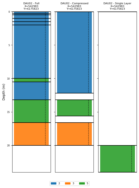
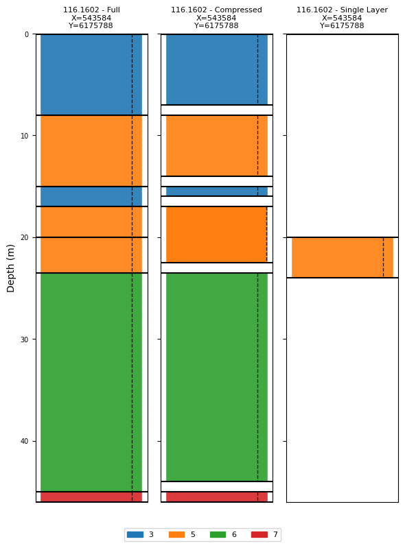
• Full: every logged layer is kept as a separate interval. Gives the most detail but may include very thin intervals.

• Compressed: adjacent intervals with the same (or similar) class are merged, and uncertain transition zones are omitted. A good compromise between detail and robustness.

• Single-layer: only one key interval is used (e.g. the target horizon). Useful when only one depth range matters or when uncertainty is high.

All three representations can be used interchangeably in INTEGRATE.

P_single = 0.9  # Default confidence probability for each observed class

# ---- Borehole DAU02 --------------------------------------------------------

BH_DAU02_full = {
    'name': 'DAU02 - Full',
    'X': 542983.01,
    'Y': 6175822.76,
    # Every logged layer (10 intervals, including thin transition zones)
    'depth_top':    [0,   0.3, 0.5,  1,   1.5,  2,  10,  10.5, 13.2, 16.6],
    'depth_bottom': [0.3, 0.5, 1,    1.5, 2,   10,  10.5, 13.2, 16.6, 20  ],
    'class_obs':    [2,   2,   2,    2,   2,    2,   5,    2,    5,    3   ],
    'class_prob':   [P_single] * 10,
}

BH_DAU02_compressed = {
    'name': 'DAU02 - Compressed',
    'X': 542983.01,
    'Y': 6175822.76,
    # Merged intervals: thin transition zones removed (3 intervals)
    'depth_top':    [0,    13.2, 16.6],
    'depth_bottom': [12.2, 15.6, 20  ],
    'class_obs':    [2,    5,    3   ],
    'class_prob':   [P_single] * 3,
}

BH_DAU02_single = {
    'name': 'DAU02 - Single Layer',
    'X': 542983.01,
    'Y': 6175822.76,
    # Only the target interval: sand/gravel at 20–24 m
    'depth_top':    [20],
    'depth_bottom': [24],
    'class_obs':    [5],
    'class_prob':   [P_single],
}

# ---- Borehole 116.1602 ------------------------------------------------------

BH_116_full = {
    'name': '116.1602 - Full',
    'X': 543584.098,
    'Y': 6175788.478,
    # Every logged layer (7 intervals)
    'depth_top':    [0,   8,  15, 17, 20,   23.5, 45],
    'depth_bottom': [8,  15,  17, 20, 23.5, 45,   46],
    'class_obs':    [3,   5,   3,  5,  5,    6,    7 ],
    'class_prob':   [P_single] * 7,
}

BH_116_compressed = {
    'name': '116.1602 - Compressed',
    'X': 543584.098,
    'Y': 6175788.478,
    # Merged intervals; transition zones at 15–17 m and 23.5 m retained
    # Note: higher confidence (0.99) for the 17–22.5 m interval
    'depth_top':    [0,   8,  15,  17,   23.5, 45],
    'depth_bottom': [7,  14,  16,  22.5, 44,   46],
    'class_obs':    [3,   5,   3,   5,    6,    7 ],
    'class_prob':   [P_single, P_single, P_single, 0.99, P_single, P_single],
}

BH_116_single = {
    'name': '116.1602 - Single Layer',
    'X': 543584.098,
    'Y': 6175788.478,
    # Only the sand/gravel interval at 20–24 m
    'depth_top':    [20],
    'depth_bottom': [24],
    'class_obs':    [5],
    'class_prob':   [P_single],
}

print("DAU02 intervals (full):       ", len(BH_DAU02_full['depth_top']))
print("DAU02 intervals (compressed): ", len(BH_DAU02_compressed['depth_top']))
print("DAU02 intervals (single):     ", len(BH_DAU02_single['depth_top']))
print()
print("116.1602 intervals (full):       ", len(BH_116_full['depth_top']))
print("116.1602 intervals (compressed): ", len(BH_116_compressed['depth_top']))
print("116.1602 intervals (single):     ", len(BH_116_single['depth_top']))

DAU02 intervals (full):        10
DAU02 intervals (compressed):  3
DAU02 intervals (single):      1

116.1602 intervals (full):        7
116.1602 intervals (compressed):  6
116.1602 intervals (single):      1

3. Visualising boreholes

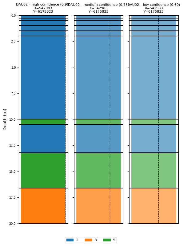
ig.plot_boreholes(W) draws a lithology column for each borehole:

• Each interval is a coloured bar; bar transparency reflects class_prob.

• A dashed vertical line shows the confidence probability.

• When a prior HDF5 file is supplied (f_prior_h5), the plot uses the class names and colours stored in the prior (instead of numeric IDs).

• Multiple representations of the same borehole can be compared by placing them side-by-side in one list.

# Plot the three representations of DAU02 together (no prior → numeric class IDs)
ig.plot_boreholes(
    [BH_DAU02_full, BH_DAU02_compressed, BH_DAU02_single],
)
plt.suptitle('DAU02 – three levels of detail', y=1.01)
if hardcopy:
    plt.savefig('boreholes_DAU02_comparison.png', dpi=200, bbox_inches='tight')
plt.show()

<Figure size 640x480 with 0 Axes>

# Same for borehole 116.1602
ig.plot_boreholes(
    [BH_116_full, BH_116_compressed, BH_116_single],
)
plt.suptitle('116.1602 – three levels of detail', y=1.01)
if hardcopy:
    plt.savefig('boreholes_116_comparison.png', dpi=200, bbox_inches='tight')
plt.show()

<Figure size 640x480 with 0 Axes>

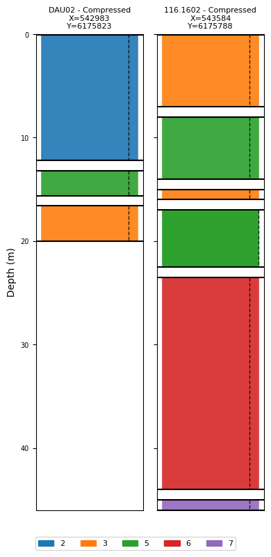
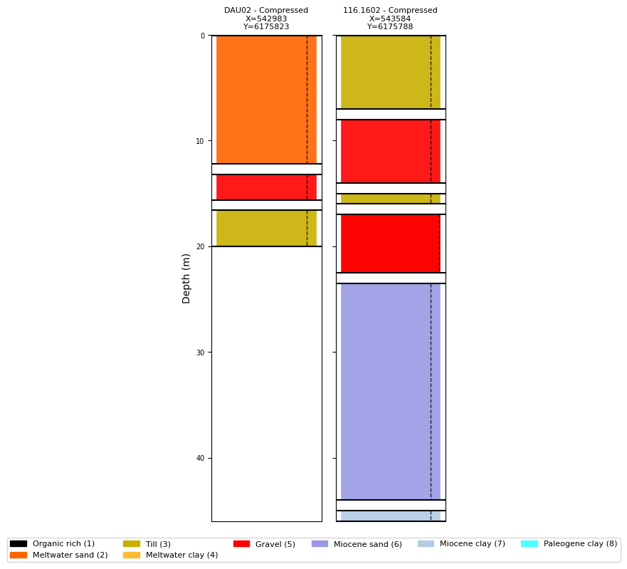
# Plot the two compressed boreholes that will be used in the integration workflow
BHOLES = [BH_DAU02_compressed, BH_116_compressed]
ig.plot_boreholes(BHOLES)
if hardcopy:
    plt.savefig('boreholes_compressed.png', dpi=200, bbox_inches='tight')
plt.show()

<Figure size 640x480 with 0 Axes>

4. Saving and loading borehole data

Borehole dictionaries (or lists of them) can be persisted to JSON with ig.write_borehole() and restored with ig.read_borehole().

• A single dict is written/read as a JSON object { ... }.

• A list of dicts is written/read as a JSON array [ {...}, {...} ].

ig.read_borehole() accepts the JSON path and returns the same structure (single dict or list) that was written.

# --- Write individual boreholes ---
for BH in BHOLES:
    # Build a safe filename from the borehole name
    fname = 'daugaard_borehole_%s.json' % BH['name'].replace(' ', '_').replace('/', '-')
    ig.write_borehole(BH, fname, showInfo=1)

# --- Write all boreholes together in one file ---
ig.write_borehole(BHOLES, 'daugaard_boreholes.json', showInfo=1)

write_borehole: wrote 1 borehole(s) to daugaard_borehole_DAU02_-_Compressed.json
write_borehole: wrote 1 borehole(s) to daugaard_borehole_116.1602_-_Compressed.json
write_borehole: wrote 2 borehole(s) to daugaard_boreholes.json

'daugaard_boreholes.json'

# --- Read back a single borehole ---
BH_loaded = ig.read_borehole(
    'daugaard_borehole_%s.json' % BHOLES[0]['name'].replace(' ', '_').replace('/', '-'),
    showInfo=1)

print('name     :', BH_loaded['name'])
print('X, Y     :', BH_loaded['X'], BH_loaded['Y'])
print('intervals:', list(zip(BH_loaded['depth_top'], BH_loaded['depth_bottom'])))
print('class_obs:', BH_loaded['class_obs'])
print('class_prob:', BH_loaded['class_prob'])

read_borehole: read 1 borehole(s) from daugaard_borehole_DAU02_-_Compressed.json
name     : DAU02 - Compressed
X, Y     : 542983.01 6175822.76
intervals: [(0, 12.2), (13.2, 15.6), (16.6, 20)]
class_obs: [2, 5, 3]
class_prob: [0.9, 0.9, 0.9]

# --- Read back all boreholes at once ---
BHOLES_loaded = ig.read_borehole('daugaard_boreholes.json', showInfo=1)
for BH in BHOLES_loaded:
    print(f"  {BH['name']:35s}  {len(BH['depth_top'])} intervals  "
          f"X={BH['X']:.1f}  Y={BH['Y']:.1f}")

read_borehole: read 2 borehole(s) from daugaard_boreholes.json
  DAU02 - Compressed                   3 intervals  X=542983.0  Y=6175822.8
  116.1602 - Compressed                6 intervals  X=543584.1  Y=6175788.5

5. Controlling observation confidence with class_prob

class_prob is the probability assigned to the observed class at each depth interval. The remaining probability mass (1 - class_prob) is distributed equally over all other classes.

Value	Meaning
1.0	Certain observation – no other class is possible
0.9	High confidence (typical field data)
0.7	Moderate confidence (ambiguous log signature)
0.5	Random guess – no information

A value below 1/n_classes is mathematically nonsensical (the observed class becomes less likely than the alternatives).

The transparency of each bar in ig.plot_boreholes() reflects class_prob, making it easy to see which intervals carry strong vs. weak information.

# Demonstrate the effect of different confidence levels on the same borehole

BH_high = dict(BH_DAU02_full)
BH_high['name'] = 'DAU02 – high confidence (0.99)'
BH_high['class_prob'] = [0.99] * len(BH_high['class_obs'])

BH_medium = dict(BH_DAU02_full)
BH_medium['name'] = 'DAU02 – medium confidence (0.75)'
BH_medium['class_prob'] = [0.75] * len(BH_medium['class_obs'])

BH_low = dict(BH_DAU02_full)
BH_low['name'] = 'DAU02 – low confidence (0.60)'
BH_low['class_prob'] = [0.60] * len(BH_low['class_obs'])

ig.plot_boreholes([BH_high, BH_medium, BH_low])
plt.suptitle('Effect of class_prob on visualisation', y=1.01)
if hardcopy:
    plt.savefig('boreholes_confidence_comparison.png', dpi=200, bbox_inches='tight')
plt.show()

<Figure size 640x480 with 0 Axes>

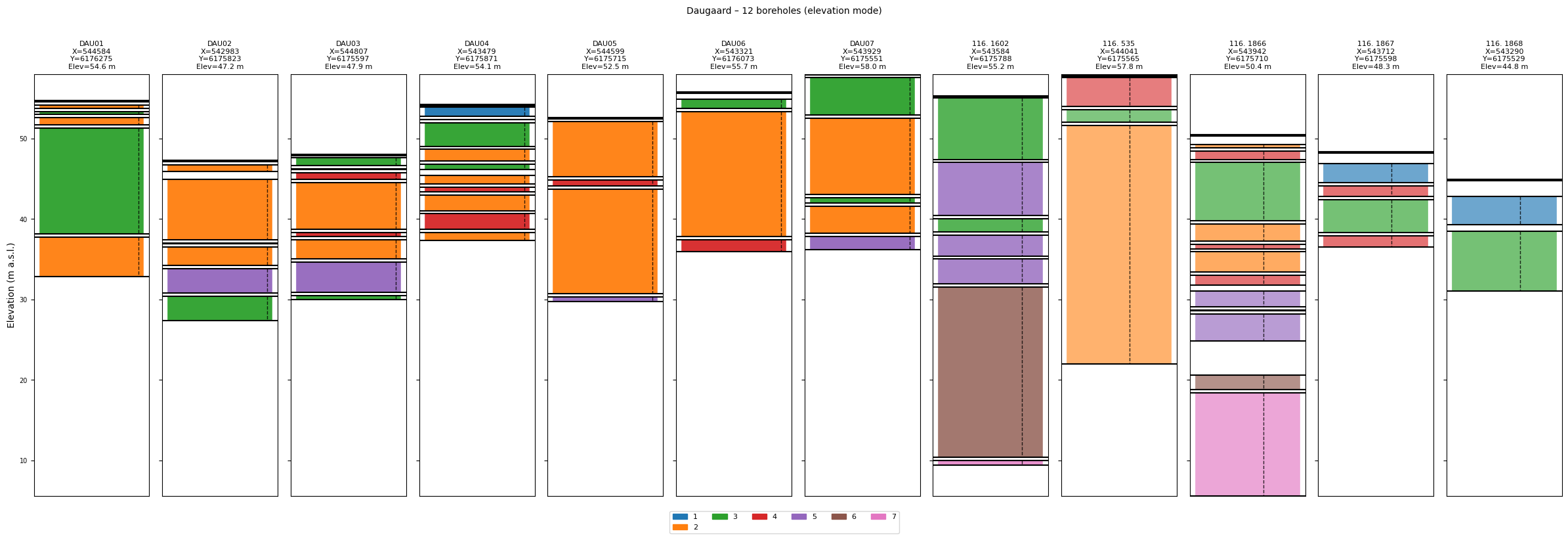
6. Loading and visualising the full Daugaard borehole dataset

The Daugaard case ships with a JSON file containing 12 boreholes with elevation information (daugaard_12boreholes.json). Because each borehole dict contains an elevation key, ig.plot_boreholes() automatically switches to elevation mode: the shared Y-axis shows metres above sea level rather than depth below surface, and every borehole stick is positioned at its ground-surface elevation. This gives a more realistic cross-section view of the subsurface.

# Download the borehole JSON file (skipped silently if already present)
ig.get_case_data(case='DAUGAARD', filelist=['daugaard_12boreholes.json'])

# Load all 12 boreholes
BHOLES_12 = ig.read_borehole('daugaard_12boreholes.json', showInfo=1)

print("Loaded %d boreholes:" % len(BHOLES_12))
for BH in BHOLES_12:
    print("  %-15s  elev=%.1f m  %d intervals" % (
        BH['name'], BH.get('elevation', 0), len(BH['depth_top'])))

Getting data for case: DAUGAARD
--> Got data for case: DAUGAARD
read_borehole: read 12 borehole(s) from daugaard_12boreholes.json
Loaded 12 boreholes:
  DAU01            elev=54.6 m  5 intervals
  DAU02            elev=47.2 m  6 intervals
  DAU03            elev=47.9 m  8 intervals
  DAU04            elev=54.1 m  10 intervals
  DAU05            elev=52.5 m  4 intervals
  DAU06            elev=55.7 m  3 intervals
  DAU07            elev=58.0 m  5 intervals
  116. 1602        elev=55.2 m  7 intervals
  116. 535         elev=57.8 m  3 intervals
  116. 1866        elev=50.4 m  12 intervals
  116. 1867        elev=48.3 m  4 intervals
  116. 1868        elev=44.8 m  2 intervals

# Plot all 12 boreholes – elevation mode is triggered automatically
ig.plot_boreholes(BHOLES_12, title='Daugaard – 12 boreholes (elevation mode)')
if hardcopy:
    plt.savefig('boreholes_daugaard_12.png', dpi=200, bbox_inches='tight')
plt.show()

<Figure size 640x480 with 0 Axes>

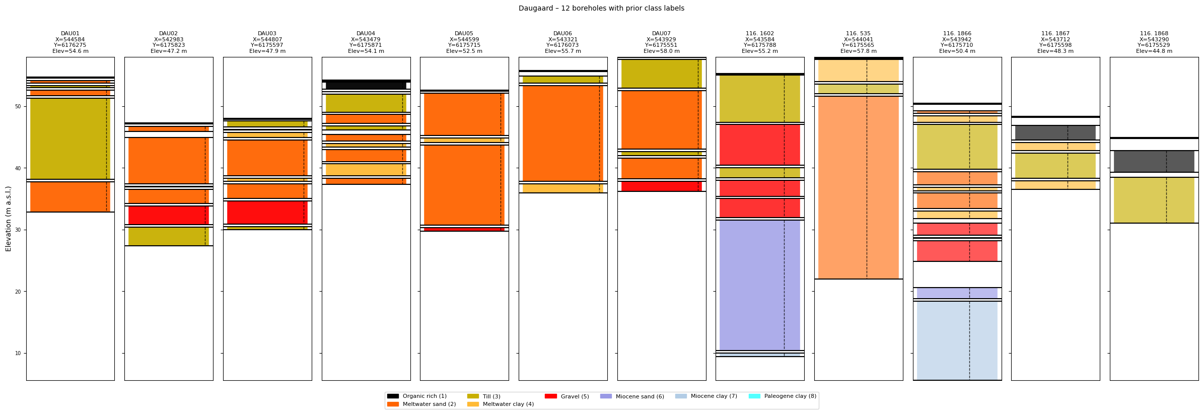
# Plot again with prior class names and colours (if the prior file is available)
import glob
prior_candidates = sorted(glob.glob('daugaard_merged_prior_N*.h5'))
if prior_candidates:
    f_prior_h5_12 = prior_candidates[-1]
    print("Using prior for class labels: %s" % f_prior_h5_12)
    ig.plot_boreholes(BHOLES_12, f_prior_h5_12,
                      title='Daugaard – 12 boreholes with prior class labels')
    if hardcopy:
        plt.savefig('boreholes_daugaard_12_prior.png', dpi=200, bbox_inches='tight')
    plt.show()
else:
    print("No merged prior file found – skipping plot with prior class labels.")

Using prior for class labels: daugaard_merged_prior_N2000000.h5

<Figure size 640x480 with 0 Axes>

7. Integrating boreholes into the prior/data workflow

Before borehole data can be used in rejection sampling, two steps are needed:

Step A – Get the prior and data files The prior HDF5 must already contain a discrete lithology model (e.g. /M2). The data HDF5 holds observed geophysical data and the survey geometry.

Step B – ``ig.save_borehole_data()`` This high-level function does everything in one call:

1. Extracts the prior lithology ensemble (/M{im_prior}) and computes, for each borehole interval, the mode class across all realisations.

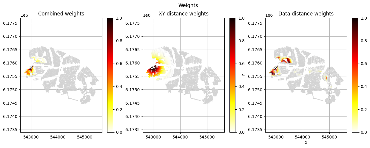
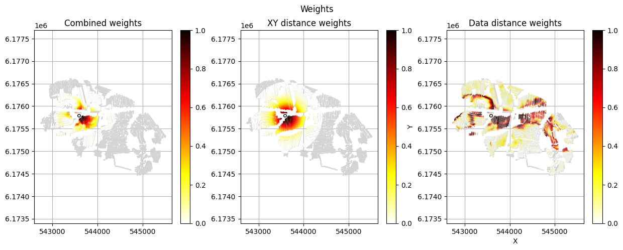
2. Builds a probability matrix P_obs (n_classes × n_intervals) from the observed class IDs and class_prob values.

3. Spatially extrapolates the point observation across the survey grid using a distance-based temperature weighting:

   • Within r_data metres: observation strength = 1 (full weight).

   • Beyond r_dis metres: weight approaches zero (observation ignored).

   • Between r_data and r_dis: smooth Gaussian fade-out.

4. Saves the gridded observation as a new dataset in the data HDF5 file and returns its ID so it can be referenced in ig.integrate_rejection().

Key parameters of ig.save_borehole_data():

Parameter	Default	Description
im_prior	2	Index of discrete model in prior (e.g. /M2)
r_data	2	Inner radius (m): full observation strength
r_dis	300	Outer radius (m): weight drops to ~0 beyond this
doPlot	False	Plot spatial weight maps for inspection
parallel	False	Enable multiprocessing for large prior ensembles

# Load the DAUGAARD case files (prior + electromagnetic data)
case = 'DAUGAARD'
f_xlsx_files = ['daugaard_standard.xlsx', 'daugaard_valley.xlsx']

# Download example data if not already present
ig.get_case_data(case=case, filelist=f_xlsx_files)
files = ig.get_case_data(case=case)
f_data_h5 = files[0]
file_gex = ig.get_gex_file_from_data(f_data_h5)

print("Data file : %s" % f_data_h5)
print("GEX file  : %s" % file_gex)

# Make a working copy so the original file is not modified
f_data_old_h5 = f_data_h5
f_data_h5 = f_data_h5.replace('.h5', '_BH.h5')
ig.copy_hdf5_file(f_data_old_h5, f_data_h5)

Getting data for case: DAUGAARD
--> Got data for case: DAUGAARD
Getting data for case: DAUGAARD
--> Got data for case: DAUGAARD
Data file : DAUGAARD_AVG.h5
GEX file  : TX07_20231016_2x4_RC20-33.gex

'DAUGAARD_AVG_BH.h5'

# Load the pre-computed merged prior (if available) or build it from the xlsx files.
# For the integration step we need a prior with electromagnetic forward data (/D1)
# AND a discrete lithology model (/M2).
#
# If you have not yet run integrate_workflow.py (or the prior files are missing),
# you can generate them with geoprior1d:
#
#   from geoprior1d import geoprior1d
#   N = 100000
#   f_prior_h5_list = []
#   for file_xlsx in f_xlsx_files:
#       fname = file_xlsx.split('.')[0]
#       f_prior_h5, _ = geoprior1d(file_xlsx, Nreals=N, dz=1, dmax=90,
#                                   output_file='%s_prior_N%d.h5' % (fname, N))
#       f_prior_h5_list.append(f_prior_h5)
#   f_prior_h5 = ig.merge_prior(f_prior_h5_list,
#                                f_prior_merged_h5='daugaard_merged_prior_N%d.h5' % N)
#   f_prior_h5 = ig.prior_data_gaaem(f_prior_h5, file_gex, doMakePriorCopy=False)
#
# Here we assume the prior already exists (produced by integrate_workflow.py):
import glob
prior_candidates = sorted(glob.glob('daugaard_merged_prior_N*.h5'))
if prior_candidates:
    f_prior_h5 = prior_candidates[-1]   # pick the largest N available
    print("Using existing prior: %s" % f_prior_h5)
else:
    raise FileNotFoundError(
        "No merged prior file found. "
        "Run integrate_workflow.py first to generate the prior, "
        "or follow the commented block above.")

Using existing prior: daugaard_merged_prior_N2000000.h5

Plot boreholes with prior class names and colours

Once the prior HDF5 is available, ig.plot_boreholes() can read the class names and colour map stored in the prior and use them instead of numeric IDs. This makes the lithology column much easier to interpret.

# Plot compressed boreholes with class metadata from the prior
ig.plot_boreholes(BHOLES, f_prior_h5)
if hardcopy:
    plt.savefig('boreholes_with_prior_classes.png', dpi=200, bbox_inches='tight')
plt.show()

<Figure size 640x480 with 0 Axes>

Compute and save borehole data for rejection sampling

We call ig.save_borehole_data() once per borehole. The function returns:

• id_prior: dataset index of the mode-class array saved in the prior file

• id_out : dataset index of the gridded observation saved in the data file

The returned id_out values are later passed to ig.integrate_rejection() via id_use to select which data types to include in the inversion.

im_prior = 2    # Lithology model index (corresponds to /M2 in the prior HDF5)
r_data   = 4    # Inner radius (m): full observation strength out to this distance
r_dis    = 300  # Outer radius (m): weight fades to ~0 at this distance

id_borehole_list = []
for BH in BHOLES:
    id_prior, id_out = ig.save_borehole_data(
        f_prior_h5, f_data_h5, BH,
        im_prior=im_prior,
        r_data=r_data,
        r_dis=r_dis,
        doPlot=True,   # Creates spatial weight maps – useful for quality control
        showInfo=1)
    id_borehole_list.append(id_out)
    print("  %-35s → prior D%d, data D%d" % (BH['name'], id_prior, id_out))

print()
print("Borehole data IDs in data file:", id_borehole_list)

prior_data_borehole: borehole=DAU02 - Compressed  method=mode_probability
compute_P_obs_sparse: Processing 4000000 realizations, 3 intervals
Using id=2
Trying to write D2 to DAUGAARD_AVG_BH.h5
Adding group DAUGAARD_AVG_BH.h5:D2
save_borehole_data: DAU02 - Compressed  →  prior D5, data D2
  DAU02 - Compressed                  → prior D5, data D2
prior_data_borehole: borehole=116.1602 - Compressed  method=mode_probability
compute_P_obs_sparse: Processing 4000000 realizations, 6 intervals
Using id=3
Trying to write D3 to DAUGAARD_AVG_BH.h5
Adding group DAUGAARD_AVG_BH.h5:D3
save_borehole_data: 116.1602 - Compressed  →  prior D6, data D3
  116.1602 - Compressed               → prior D6, data D3

Borehole data IDs in data file: [2, 3]

8. Using borehole data in rejection sampling

After ig.save_borehole_data() the data HDF5 contains:

• Dataset 1 (/D1): the electromagnetic (tTEM) observed data

• Dataset 2+ (/D2, /D3, …): the gridded borehole observations

ig.integrate_rejection() accepts an id_use list to select which datasets participate in the joint inversion. Common choices:

id_use = [1] # EM data only id_use = id_borehole_list # Borehole data only id_use = [1] + id_borehole_list # EM + all boreholes (joint)

The code below shows the pattern without executing the inversion (which requires the full prior ensemble and can take several minutes).

# Example: how to call integrate_rejection with borehole data
# (This cell is illustrative – uncomment to run the full inversion)

nr    = 1000     # Number of accepted realisations to retain per data point
N_use = None     # Number of prior realisations to use (None = all)

# --- EM data only ---
# f_post_em = ig.integrate_rejection(
#     f_prior_h5, f_data_h5, 'post_EM_only.h5',
#     id_use=[1], nr=nr, N_use=N_use, showInfo=1, updatePostStat=True)

# --- Borehole data only ---
# f_post_bh = ig.integrate_rejection(
#     f_prior_h5, f_data_h5, 'post_BH_only.h5',
#     id_use=id_borehole_list, nr=nr, N_use=N_use, showInfo=1, updatePostStat=True)

# --- Joint inversion: EM + boreholes ---
# f_post_joint = ig.integrate_rejection(
#     f_prior_h5, f_data_h5, 'post_EM_BH_joint.h5',
#     id_use=[1] + id_borehole_list, nr=nr, N_use=N_use, showInfo=1, updatePostStat=True)

print("id_use options:")
print("  EM only        : id_use = [1]")
print("  Boreholes only : id_use = %s" % id_borehole_list)
print("  Joint (EM+BH)  : id_use = %s" % ([1] + id_borehole_list))

id_use options:
  EM only        : id_use = [1]
  Boreholes only : id_use = [2, 3]
  Joint (EM+BH)  : id_use = [1, 2, 3]