INTEGRATE on ESBJERG data¶

[1]:

try:
    # Check if the code is running in an IPython kernel (which includes Jupyter notebooks)
    get_ipython()
    # If the above line doesn't raise an error, it means we are in a Jupyter environment
    # Execute the magic commands using IPython's run_line_magic function
    get_ipython().run_line_magic('load_ext', 'autoreload')
    get_ipython().run_line_magic('autoreload', '2')
except:
    # If get_ipython() raises an error, we are not in a Jupyter environment
    # # # # # #%load_ext autoreload
    # # # # # #%autoreload 2
    pass

[2]:

import integrate as ig
import numpy as np
import matplotlib.pyplot as plt
# check if parallel computations can be performed
parallel = ig.use_parallel(showInfo=1)
hardcopy = True

Notebook detected. Parallel processing is OK

[3]:

N=5000000
N=50000
case = 'ESBJERG'
files = ig.get_case_data(case=case)
f_data_h5 = files[0]
file_gex= ig.get_gex_file_from_data(f_data_h5)

print("Using data file: %s" % f_data_h5)
print("Using GEX file: %s" % file_gex)

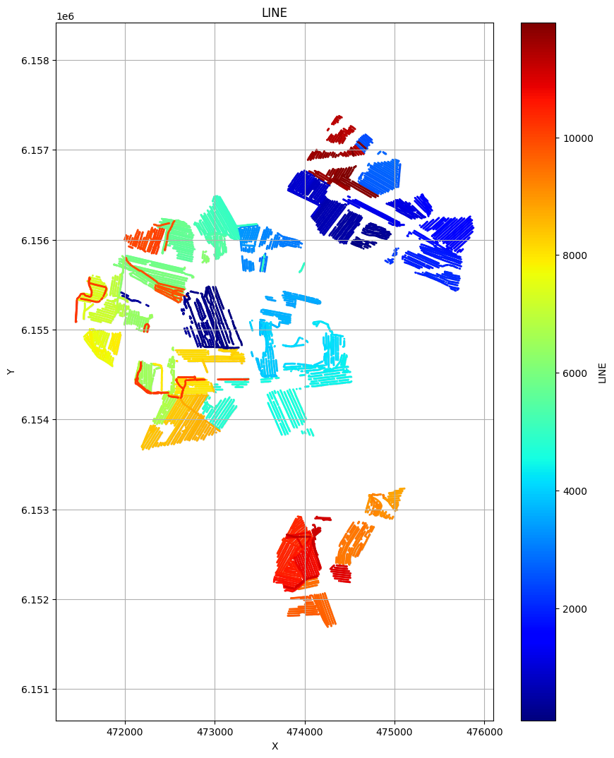
ig.plot_geometry(f_data_h5, pl='LINE')
X, Y, LINE, ELEVATION = ig.get_geometry(f_data_h5)

Getting data for case: ESBJERG
Downloading ESBJERG_ALL.h5
Downloaded ESBJERG_ALL.h5
Downloading TX07_20230906_2x4_RC20-33.gex
Downloaded TX07_20230906_2x4_RC20-33.gex
Downloading README_ESBJERG
Downloaded README_ESBJERG
--> Got data for case: ESBJERG
Using data file: ESBJERG_ALL.h5
Using GEX file: TX07_20230906_2x4_RC20-33.gex
f_data_h5=ESBJERG_ALL.h5

../_images/notebooks_integrate_esbjerg_3_1.png

1. Setup the prior model (\(\rho(\mathbf{m},\mathbf{d})\)¶

In this example a simple layered prior model will be considered

1a. first, a sample of the prior model parameters, \(\rho(\mathbf{m})\), will be generated¶

[4]:

# Layered model
f_prior_h5 = ig.prior_model_layered(N=N,lay_dist='chi2', NLAY_deg=3, RHO_min=1, RHO_max=500)
f_prior_h5 = ig.prior_model_layered(N=N,lay_dist='uniform', NLAY_min=1, NLAY_max=8, RHO_min=1, RHO_max=500)

# Plot some summary statistics of the prior model
#ig.plot_prior_stats(f_prior_h5)

File PRIOR_CHI2_NF_3_log-uniform_N50000.h5 does not exist.

File PRIOR_UNIFORM_NL_1-8_log-uniform_N50000.h5 does not exist.

1b. Then, a corresponding sample of \(\rho(\mathbf{d})\), will be generated¶

[5]:

f_prior_data_h5 = ig.prior_data_gaaem(f_prior_h5, file_gex, parallel=parallel, showInfo=0)

Using file_basename=TX07_20230906_2x4_RC20-33
prior_data_gaaem: Using 32 parallel threads.

prior_data_gaaem: Time= 70.3s/50000 soundings.  1.4ms/sounding, 711.3it/s

[6]:

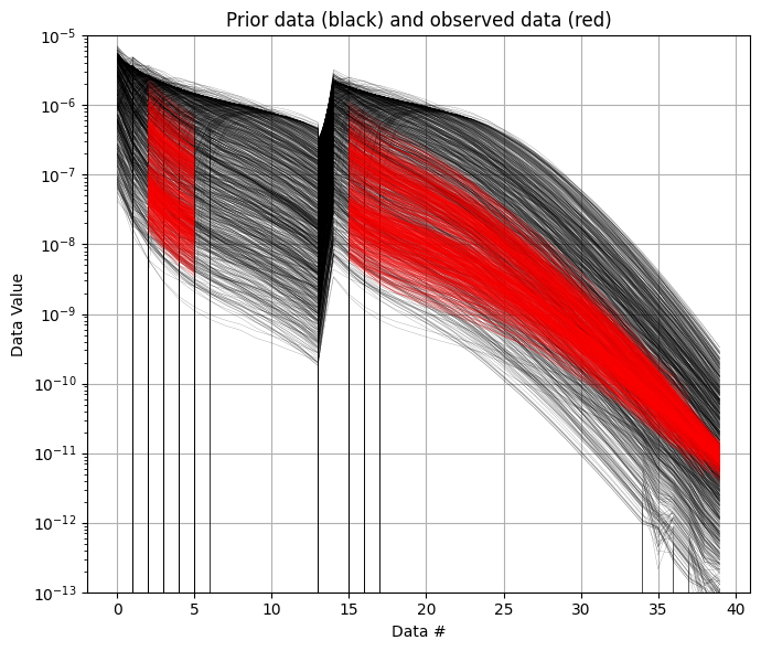
ig.plot_data_prior(f_prior_data_h5,f_data_h5,nr=1000,alpha=1, ylim=[1e-13,1e-5], hardcopy=hardcopy)

../_images/notebooks_integrate_esbjerg_9_0.png

[6]:

True

Sample the posterior \(\sigma(\mathbf{m})\)¶

The posterior distribution is sampling using the extended rejection sampler.

[7]:

N_use = N
f_post_h5 = ig.integrate_rejection(f_prior_data_h5,
                                   f_data_h5,
                                   N_use = N_use,
                                   showInfo=1,
                                   Ncpu = 10,
                                   parallel=parallel)

Loading data from ESBJERG_ALL.h5. Using data types: [1]
  - D1: id_prior=1,    gaussian, Using 28061/40 data
Loading prior data from PRIOR_UNIFORM_NL_1-8_log-uniform_N50000_TX07_20230906_2x4_RC20-33_Nh280_Nf12.h5. Using prior data ids: [1]
  - /D1:  N,nd = 50000/40
<--INTEGRATE_REJECTION-->
f_prior_h5=PRIOR_UNIFORM_NL_1-8_log-uniform_N50000_TX07_20230906_2x4_RC20-33_Nh280_Nf12.h5, f_data_h5=ESBJERG_ALL.h5
f_post_h5=/mnt/space/space_au11687/PROGRAMMING/integrate_module/examples/POST_PRIOR_UNIFORM_NL_1-8_log-uniform_N50000_TX07_20230906_2x4_RC20-33_Nh280_Nf12_Nu50000_aT1.h5

integrate_rejection: Time=181.3s/28061 soundings,  6.5ms/sounding, 154.7it/s. T_av=59.9, EV_av=-74.7
Computing posterior statistics for 28061 of 28061 data points

Creating /M1/Mean in /mnt/space/space_au11687/PROGRAMMING/integrate_module/examples/POST_PRIOR_UNIFORM_NL_1-8_log-uniform_N50000_TX07_20230906_2x4_RC20-33_Nh280_Nf12_Nu50000_aT1.h5
Creating /M1/Median in /mnt/space/space_au11687/PROGRAMMING/integrate_module/examples/POST_PRIOR_UNIFORM_NL_1-8_log-uniform_N50000_TX07_20230906_2x4_RC20-33_Nh280_Nf12_Nu50000_aT1.h5
Creating /M1/Std in /mnt/space/space_au11687/PROGRAMMING/integrate_module/examples/POST_PRIOR_UNIFORM_NL_1-8_log-uniform_N50000_TX07_20230906_2x4_RC20-33_Nh280_Nf12_Nu50000_aT1.h5
Creating /M1/LogMean in /mnt/space/space_au11687/PROGRAMMING/integrate_module/examples/POST_PRIOR_UNIFORM_NL_1-8_log-uniform_N50000_TX07_20230906_2x4_RC20-33_Nh280_Nf12_Nu50000_aT1.h5

Creating /M2/Mean in /mnt/space/space_au11687/PROGRAMMING/integrate_module/examples/POST_PRIOR_UNIFORM_NL_1-8_log-uniform_N50000_TX07_20230906_2x4_RC20-33_Nh280_Nf12_Nu50000_aT1.h5
Creating /M2/Median in /mnt/space/space_au11687/PROGRAMMING/integrate_module/examples/POST_PRIOR_UNIFORM_NL_1-8_log-uniform_N50000_TX07_20230906_2x4_RC20-33_Nh280_Nf12_Nu50000_aT1.h5
Creating /M2/Std in /mnt/space/space_au11687/PROGRAMMING/integrate_module/examples/POST_PRIOR_UNIFORM_NL_1-8_log-uniform_N50000_TX07_20230906_2x4_RC20-33_Nh280_Nf12_Nu50000_aT1.h5
Creating /M2/LogMean in /mnt/space/space_au11687/PROGRAMMING/integrate_module/examples/POST_PRIOR_UNIFORM_NL_1-8_log-uniform_N50000_TX07_20230906_2x4_RC20-33_Nh280_Nf12_Nu50000_aT1.h5

Creating /M3/Mean in /mnt/space/space_au11687/PROGRAMMING/integrate_module/examples/POST_PRIOR_UNIFORM_NL_1-8_log-uniform_N50000_TX07_20230906_2x4_RC20-33_Nh280_Nf12_Nu50000_aT1.h5
Creating /M3/Median in /mnt/space/space_au11687/PROGRAMMING/integrate_module/examples/POST_PRIOR_UNIFORM_NL_1-8_log-uniform_N50000_TX07_20230906_2x4_RC20-33_Nh280_Nf12_Nu50000_aT1.h5
Creating /M3/Std in /mnt/space/space_au11687/PROGRAMMING/integrate_module/examples/POST_PRIOR_UNIFORM_NL_1-8_log-uniform_N50000_TX07_20230906_2x4_RC20-33_Nh280_Nf12_Nu50000_aT1.h5
Creating /M3/LogMean in /mnt/space/space_au11687/PROGRAMMING/integrate_module/examples/POST_PRIOR_UNIFORM_NL_1-8_log-uniform_N50000_TX07_20230906_2x4_RC20-33_Nh280_Nf12_Nu50000_aT1.h5

Plot some statistic from \(\sigma(\mathbf{m})\)¶

[8]:

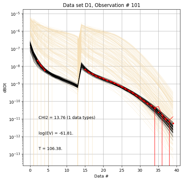
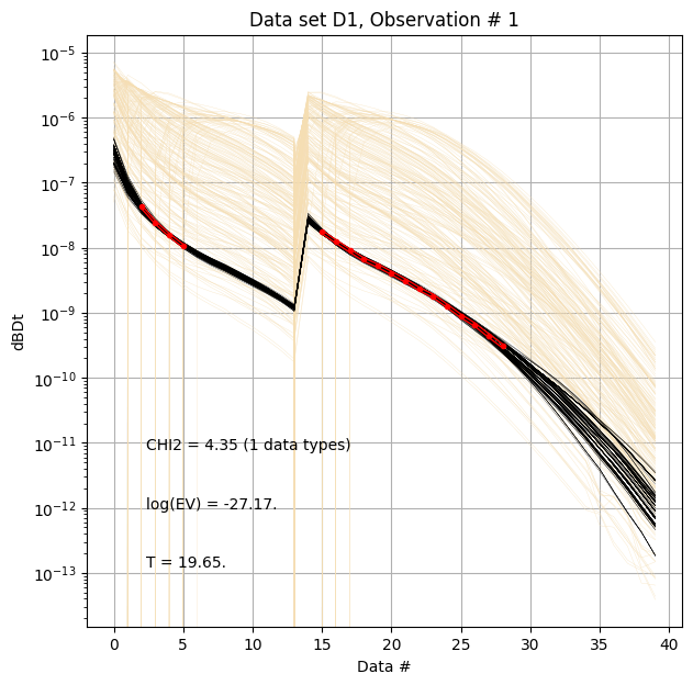
ig.plot_data_prior_post(f_post_h5, i_plot=100, hardcopy=hardcopy)
ig.plot_data_prior_post(f_post_h5, i_plot=0, hardcopy=hardcopy)

../_images/notebooks_integrate_esbjerg_13_0.png

../_images/notebooks_integrate_esbjerg_13_1.png

[9]:

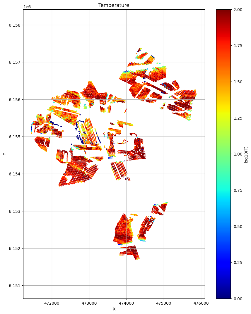
# Plot the Temperature used for inversion
ig.plot_T_EV(f_post_h5, pl='T', hardcopy=hardcopy)
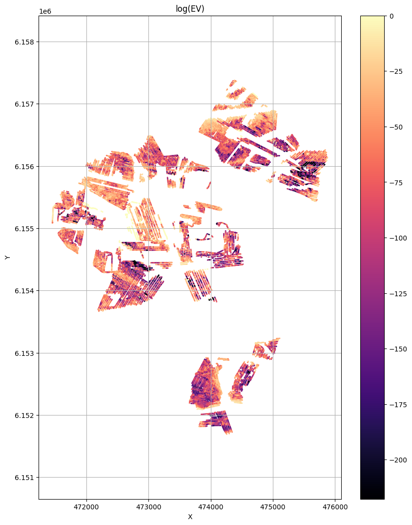
# Plot the evidnence (prior likelihood) estimated as part of inversion
ig.plot_T_EV(f_post_h5, pl='EV', hardcopy=hardcopy)

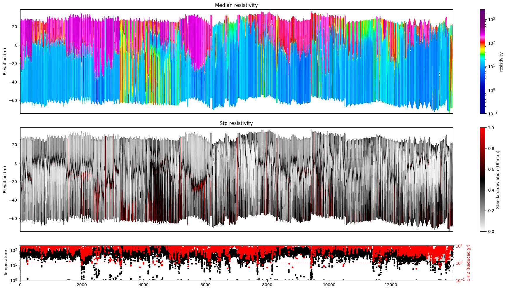
../_images/notebooks_integrate_esbjerg_14_0.png

../_images/notebooks_integrate_esbjerg_14_1.png

[10]:

# find index id of data points wher LINE==1000
#i_plot= np.where( np.abs(LINE-1200)<1  )[0]
#ig.plot_profile(f_post_h5, i1=i_plot[0], i2=i_plot[-1], im=1)
ig.plot_profile(f_post_h5, i_plot=10000, i2=14000, im=1, hardcopy=hardcopy)
#ig.plot_profile(f_post_h5, i_plot=0, i2=2000, im=2)h yg sa

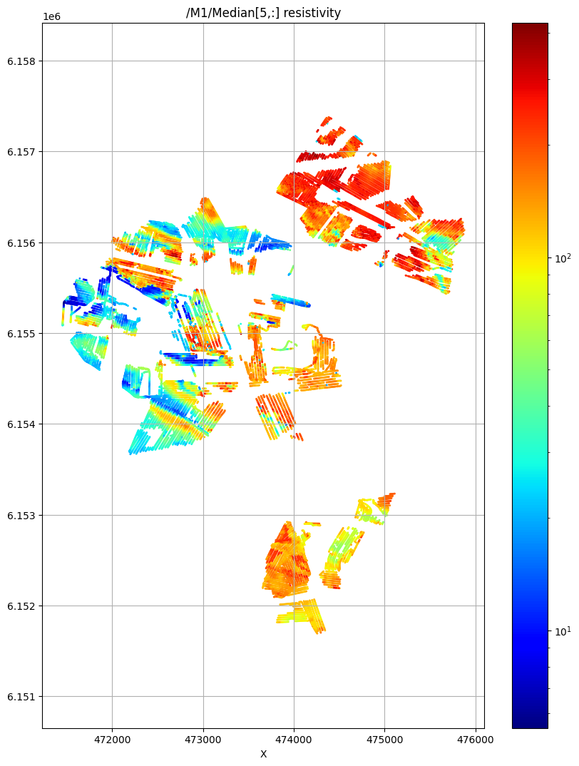
../_images/notebooks_integrate_esbjerg_15_0.png

[11]:

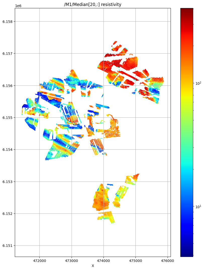
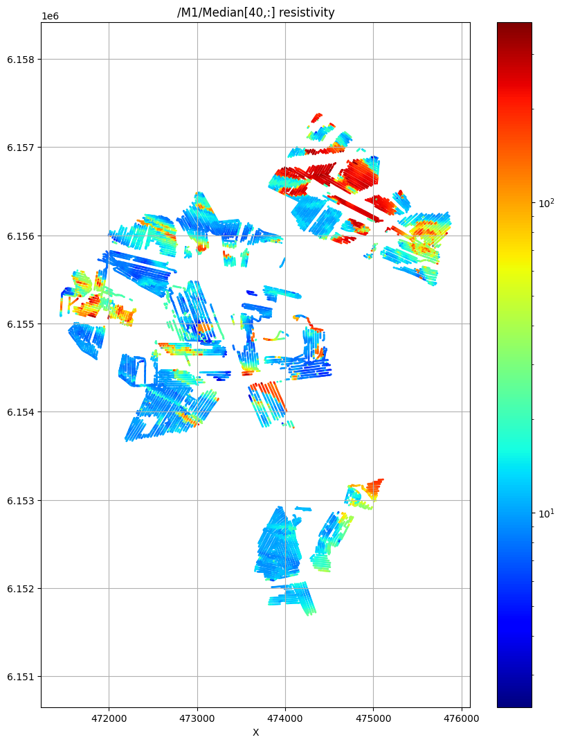
# Plot a 2D feature: Resistivity in layer 10
ig.plot_feature_2d(f_post_h5,im=1,iz=5, key='Median', uselog=1, cmap='jet', s=1, hardcopy=hardcopy)
plt.show()
ig.plot_feature_2d(f_post_h5,im=1,iz=20, key='Median', uselog=1, cmap='jet', s=1, hardcopy=hardcopy)
plt.show()
ig.plot_feature_2d(f_post_h5,im=1,iz=40, key='Median', uselog=1, cmap='jet', s=1, hardcopy=hardcopy)
plt.show()

#ig.plot_feature_2d(f_post_h5,im=1,iz=80,key='Median')

try:
    # Plot a 2D feature: The number of layers
    ig.plot_feature_2d(f_post_h5,im=2,iz=0,key='Mean', title_text = 'Number of layers', uselog=0, clim=[1,6], cmap='jet', s=1, hardcopy=hardcopy)
    plt.show()
except:
    pass

/M1/Median[5,:] resistivity

../_images/notebooks_integrate_esbjerg_16_1.png

/M1/Median[20,:] resistivity

../_images/notebooks_integrate_esbjerg_16_3.png

/M1/Median[40,:] resistivity

../_images/notebooks_integrate_esbjerg_16_5.png

../_images/notebooks_integrate_esbjerg_16_6.png

[12]:

# f_csv, f_point_csv = ig.post_to_csv(f_post_h5)